Protein structural similarity#
Proteins can be aligned by their structure instead of by their sequence. In protein structural alignment the objective is to find commonalities in the three dimensional structure which may or not relate to similarity of the primary sequence. There are many different algorithms that have been developed to perform structural alignments and also many different measurements to try to quantify the degree of structural similarity between structures. One idea that has been commonly used is to try to move and rotate one of the structures in such a way that it minimizes the distance between potentially equivalent atoms (see schematic of figure below). To achieve this, there needs to be a measurement of similarity that can be optimized and a very efficient way to search through the possible rotations and movements of the structures.
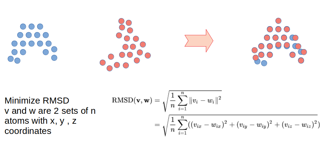
A very commonly used metric of structural similarity is called the root-mean-square deviation of atomic positions or RMSD. Given a set of two superimposed structures, RMSD is a measure of the average distance between atoms expressed in units of length, most commonly in Ångström (Å or 10−10m). RMSD can be calculated for any set of pairs of atoms depending on the application and two common sets would be all atoms or just the C-alpha atoms. There are many other algorithms to align structures that make use of other ideas such as comparing overall shapes or comparing sets of structural elements.
The similarity of protein structures can be used to predict protein function by structural homology. For example, there may be a similar pocket in both proteins which would help annotate an enzymatic activity that was unknown. Proteins with highly identical sequences will almost always have very identical structures. However, it is possible for proteins to have highly identical structures with very divergent sequences.
The Bio3D library can be used to perform and score structural alignments. In order to select a set of structures to align we can also use a Blast search to find structures that have sequences that are similar to the sequence of the kinase structure we have been analyzing (5J5X).
# Use the bio3d library
library(bio3d)

# Fetch the PDB structure with a PDB code id
pdb <- read.pdb("5J5X")

# Create a new PDB object just with A chain with the kinase domain
apdb <- trim.pdb(pdb, chain="A")

# Retrieving the protein sequence
seq <- pdbseq(apdb)

# Use Blast to query the PDB for structures of related sequences
blastResult <- blast.pdb(seq)
top.hits <- plot.blast(blastResult, cutoff=100)
The blast.pdb() function uses the sequence to find structures in the PDB that have related sequences. This information is stored in the blastResult object, which can be inspected using the plot.blast() function. This also returns a list of hits that can be stored for further queries. In this case, the hits were stored in the object top.hits.
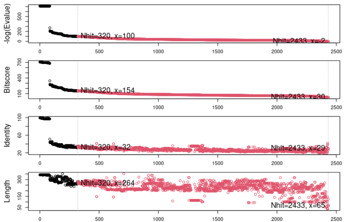
The plot above shows the visual representation of the blast results, indicating a number of highly identical sequences followed by a larger number of less related sequences. For the structural alignment we will focus on the structures having the top 10 most similar sequences based on this blast search. The structural alignment function in Bio3D takes advantage of having a multiple sequence alignment which is done via muscle.
Warning
Using the module system in R Studio
In order for R Studio to be able to use MUSCLE, you need to load the appropriate system module - how do you do this?
In R Studio we have set up a function, module(), which passes commands to the system and is able to load modules into the R Studio environment
# Load a module
module("load MUSCLE")

# List loaded modules
module("list")

# List available modules
module("avail")

# Clear loaded modules
module("purge")
# Get the PDBs for the top 10 blast hits split by chain. These will be stored in ./split_chain/. My_pdbs will hold the list of downloaded PDBs. notice that we used get.pdb() instead of read.pdb()
my_pdbs<-get.pdb(top.hits$hits[1:10], split = TRUE)

#Shortcut
my_pdbs<-get.pdb(c("7VRV_A","7JWB_A","7BYR_A","6ZP1_A","7EJ4_A","7FCD_A","7OAN_A","7WCD_C","7CAI_A","7A25_A"), split = TRUE)

# pdbaln() takes a list of PDBs to aln using MUSCLE
aln_pdbs <- pdbaln(my_pdbs)

# Structural alignment and output all fitted structures to outpath
xyz <- pdbfit(aln_pdbs, outpath="fitted")
The function pdbfit() is the function that performs the structural alignment and it is based on the minimization of the RMSD using the Kabsch algorithm. It takes advantage of the sequence alignment to have an idea of which residues are likely to be the same in different structures. The outcome of the structural alignment is a set of new PDB files that are stored in the folder “./fitted/”. These PDB files have each of the 10 structures all represented in the coordinates of the aligned structures. The pdbfit() function also returns the coordinate values for the aligned atoms, which are collapsed into a matrix format and stored in xyz. This object with coordinates can then be used in different ways to calculate and display measurements of similarity.
# Calculate RMSD
rd <- rmsd(xyz)
rd
2F7E_E 3AGM_A 3MVJ_A 6C0U_A 5VI9_A 3NX8_A 3AGL_A 1CTP_E 4WB5_A 2C1A_A
2F7E_E  0.000  0.457  0.543  4.614  1.081  0.623  0.643  1.271  0.495  0.265
3AGM_A  0.457  0.000  0.711  4.644  0.924  0.818  0.713  1.124  0.724  0.440
3MVJ_A  0.543  0.711  0.000  4.715  1.316  0.577  0.679  1.510  0.431  0.574
6C0U_A  4.614  4.644  4.715  0.000  4.770  4.663  4.672  4.892  4.679  4.663
5VI9_A  1.081  0.924  1.316  4.770  0.000  1.273  1.362  0.581  1.276  1.007
3NX8_A  0.623  0.818  0.577  4.663  1.273  0.000  0.893  1.469  0.506  0.677
3AGL_A  0.643  0.713  0.679  4.672  1.362  0.893  0.000  1.577  0.750  0.665
1CTP_E  1.271  1.124  1.510  4.892  0.581  1.469  1.577  0.000  1.467  1.208
4WB5_A  0.495  0.724  0.431  4.679  1.276  0.506  0.750  1.467  0.000  0.510
2C1A_A  0.265  0.440  0.574  4.663  1.007  0.677  0.665  1.208  0.510  0.000
# Show the RMSD values for a specific pair
rd["5VI9_A","3NX8_A"]
1.273
Exercise 9.1
Calculate the largest, mean and median RMSD values (Tip - use na.rm = TRUE to exclude NAs)
max(rd, na.rm = TRUE)
4.892

mean(rd, na.rm = TRUE)
1.46904

median(rd, na.rm = TRUE)
0.784
We can see that overall the structures tend to be highly similar (RMSD <2A). This is expected since we selected structures that are highly related by sequence. However, there are also some exceptions that suggest that there may be different conformations adopted in the different structures. To get a more visual representation of the groups of structures that are more similar to each other we can perform a clustering analysis.
# Perform hierarchical clustering of the structural similarity using as a distance the RMSDs
hc.rd <- hclust(as.dist(rd))

# Plot the hc - see how different groups are formed
plot(hc.rd)

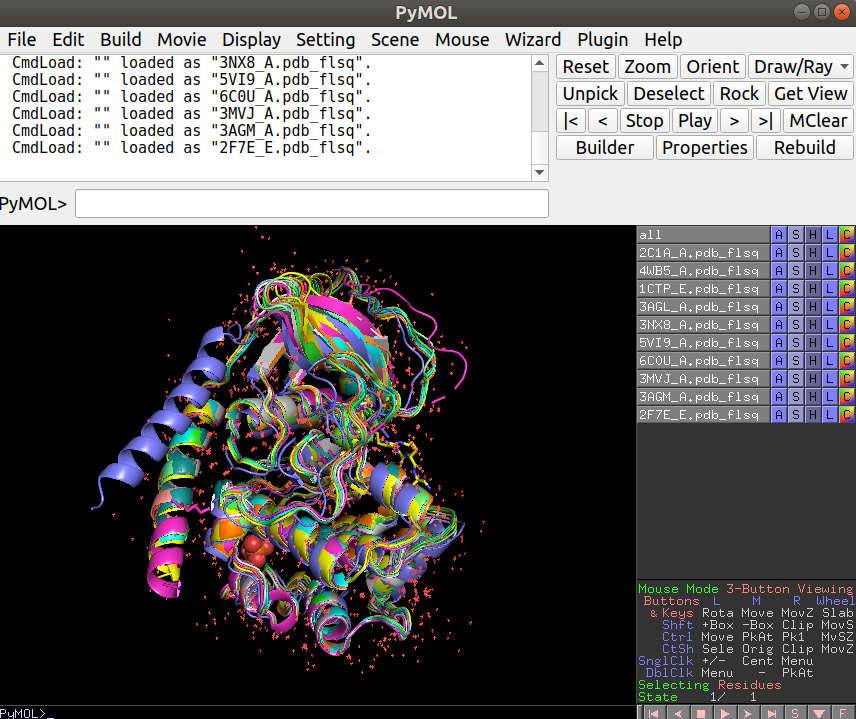
The plot above shows how the structures are grouping in terms of structural similarity. Based on these we can select some structures for visualization to better understand their differences. The superimposed structures can be found in the working directory under the folder “./fitted”. These can be downloaded to your local computer from the workbench as before and opened in Pymol together for visualization. For this you can open Pymol and simply select all the structures and drag them onto the Pymol window or through the menu select File -> Open and shift select all the structures that you want to see.
Exercise 9.2
Open the structures 6C0U_A together with any 2 other structures. What is visually different about 6C0U_A?
The N-terminal helix is in a very different location relative to the other structures
Advanced analysis - Bio3D has a set of functions that allows the user to generate a trajectory from interpolated structures that are based on a Principal Component Analysis (PCA). The following section explains how this is done and can be explored at a more advanced level.
Performing a PCA on the aligned atomic coordinates will identify the main axes of variation in the atomic coordinates. In essence, it will allow us to find the most striking differences in shape and also predict any arbitrary number of shapes along the path between these different shapes. This can be used as an hypothesis of potential dynamical behavior of the protein. The PCA on aligned atomics coordinates uses the pca.xyz() function.
# Performing PCA on the aligned structures
pca_data <- pca.xyz(xyz = xyz, rm.gaps = TRUE)

# Plot the results of PCA
plot(pca_data)
The plot below is a summary of the PCA analysis showing each of the structures represented in the lower dimension of the first 3 components. It also shows the proportion of variation in atomic coordinates that is explained by each component. These components and their degree of variation can be interpreted as possible structural dynamics.
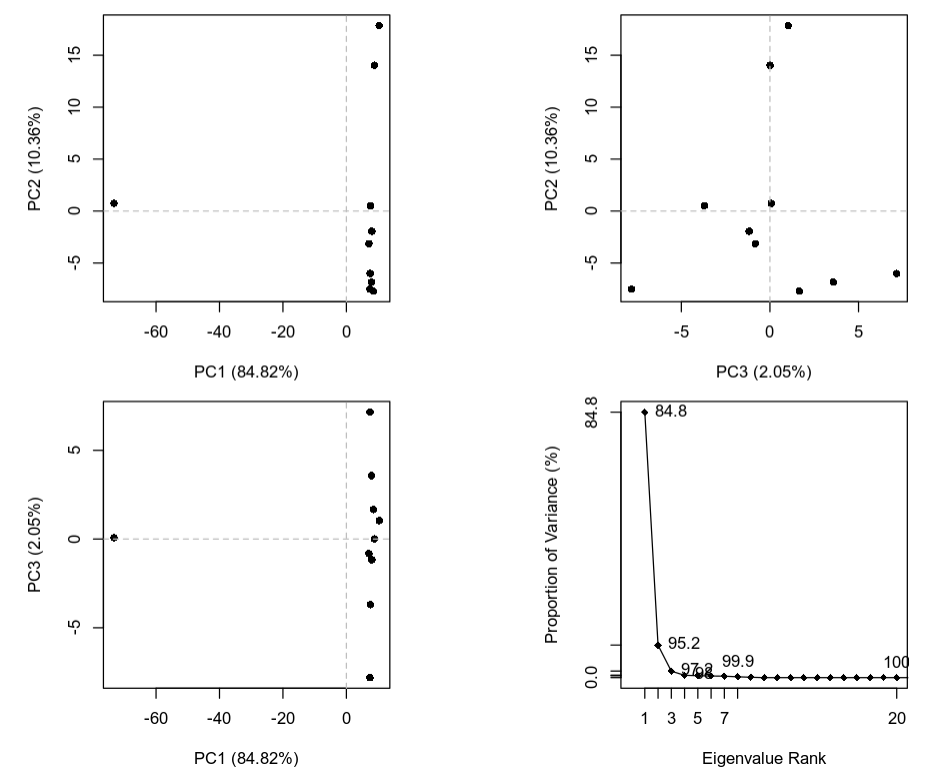
We can obtain information on the relative importance/score (PCA loadings) of each structure and each residue along these main predicted dynamical behaviors. The information for the structures is stored in pca_data$z and the equivalent for the residues in pca_data$au. For example to find the most variable residues along a specific principal component (dynamical behavior) we can plot it:
# Plot the degree of variability of each residue along PC1
plot.bio3d(pca_data$au[,1], ylab="PC1")
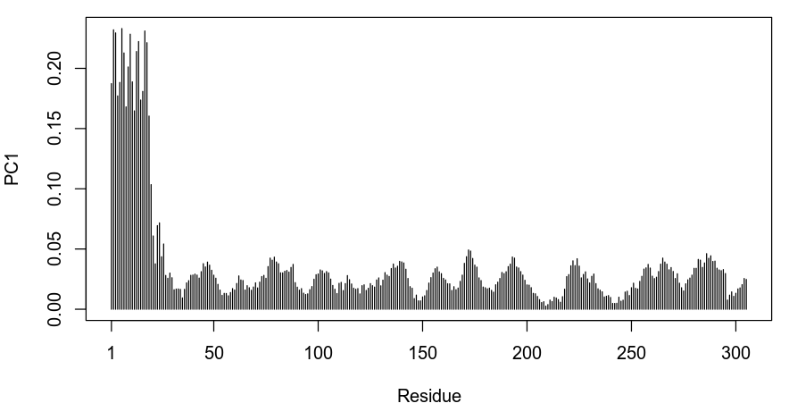
Based on the plot above we can see that the first residues in the protein are the most variable along the first component of variation. As we could have anticipated, this corresponds to the large difference in the conformation of the first helix in 6C0U_A.
Finally, we can also make an “animation” by generating several predicted structures along the axis of variation of a specific principal component. This will save the predicted structures as frames in an animation that can be visualized in Pymol.
# Make an interpolation along PC1 and save it to a file called pc1.pdb
mktrj.pca(pca_data, pc=1, file="pc1.pdb")
Exercise 9.3
Generate a similar interpolation but using instead the second principal component. Download the generated pdb file to your local computer, open it with Pymol and observe the dynamics. Try to think about what these dynamics might be for.
mktrj.pca(pca_data, pc=2, file="pc2.pdb")