Protein pockets and interaction interfaces

Protein molecules don’t work in isolation and will instead interact with other proteins, DNA/RNA or small molecules in order to be able to perform their functions. Therefore, in order to understand and study protein function we need to understand as well how they interact with other molecules. In addition, these interaction sites are used to design drugs that can alter protein behavior which is essential for rational design of therapies but also important for the development of tool compounds that are used to study biological systems .

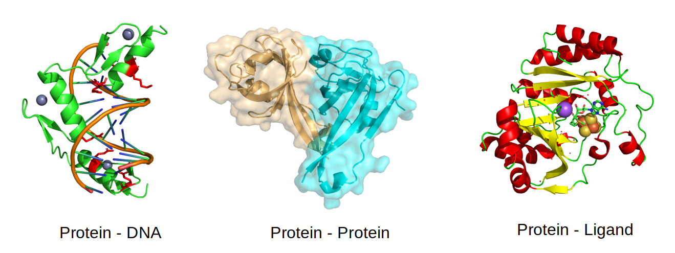
Not all protein interaction sites are the same and they can be broadly split into protein-protein interactions, protein-DNA/RNA interactions and binding sites for small molecules. Protein-protein interactions can be also classified according to properties of the interaction such as the size of the interface, the affinity or strength of interaction and its lifetime which could be transient or permanent. The interaction with small-molecules is most often occurring within well defined pockets within a protein structure, while interactions with other proteins or DNA/RNA occurs in more “flat” surfaces that are more espoused to the surface. Such binding sites within proteins are also usually classified in different types such a binding site for the substrate of the enzyme (i.e. an active site) or a binding site distal to the active site that can module enzyme function through a change in conformation (i.e. allosteric site).

The interactions are stabilized by non-covalent interactions of different types (e.g. hydrogen bonds and ionic interactions) and by the hydrophobic effect, whereby the interaction tends to be stabilized when hydrophobic amino-acids are forming an interface instead of being exposed to the solvent. Not all residues at an interface contribute equally to complex formation and understanding which residues are important and why, is key to study for example the impact of mutations. Critical interaction residues tend to be more conserved over the course of evolution. For example, the protein-DNA illustrated below is stabilized by positively charged residues in the protein (in red) with negatively charged residues in the DNA. Large protein-protein interfaces such as the one shown below are most often stabilized by buried hydrophobic amino-acids and some of the specificity can come from complementary shape. The interactions between proteins and small molecules often happens at pockets, as the one shown below, where a few key residues determine the interaction and consequent catalysis.

Identifying or predicting protein interaction sites

If we already have a protein structure bound to a protein or small molecule, we can identify the interaction surface by simply calculating the distances between atoms and then selecting residues that are close in space to the binding molecule. Alternatively, we can also calculate surface accessibility of the protein residues in the presence or absence of the binding molecule. The interface residues would be those that increase the most in their surface accessibility.

When we don’t already have a structure of binding site we can still try to predict if there are regions within the structure that may be interaction surfaces. The following properties are often used by computational methods that look for contiguous regions (i.e. patches) at the surface that could be such interface regions: * Amino acid types and their physicochemical properties - patches of amino-acids that are hydrophobic are for example more likely to be an interface region * Evolutionary properties - Critical interface residues are more conserved and may also co-evolve with the residues in the putative interacting protein * Surface accessibility and shape - Interaction regions need to be accessible and may have specific shape characteristics. * Homology with other structures - if the structure of interest has an homologous structure bound to an interacting partner the same regions within the structure of interest can be predicted as an interface region.

If you want to study these topics at a more advanced level you can read a review article that goes into more details on computational methods to predict interface residues (Xue et al. FEBS letter 2016).

Identifying interaction sites with Bio3D

Let’s start by using Bio3D to identify binding residues with the binding.site() function and the same protein kinase structure (5J5X) as before. This function can find residues between different entities (e.g. chains or small molecules) using a distance based cutoff that is set to 5 angstroms as default. When no indices are given the function will find all binding sites by default.

# Use the bio3d library
library(bio3d)

# Fetch the PDB structure with a PDB code id
pdb <- read.pdb("5J5X")

# Find all interface residues
bs <- binding.site(pdb)

The object bs will now hold the binding site information which includes the indices (bs$inds), residues names (bs$resnames) and number (bs$resno). The indices can be used in other functions of the Bio3D package such as the trim.pdb() function. To visualize the binding sites we can create a PDB file that has these binding residues and overlay them on top of the original structure for comparison.

# Extract binding atoms and print a new PDB with this
bs.pdb <- trim.pdb(pdb, inds = bs$inds)
write.pdb(bs.pdb, file = "binding_sites.pdb")

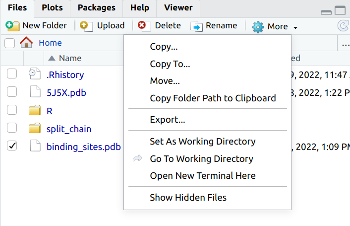
In order to visualize the binding sites we will use Pymol. You will need to download the file you have generated by selecting the file within the RStudio Workbench Files tab, then selecting More and Export. In this way you can move files from the Workbench to your local computer for viewing.

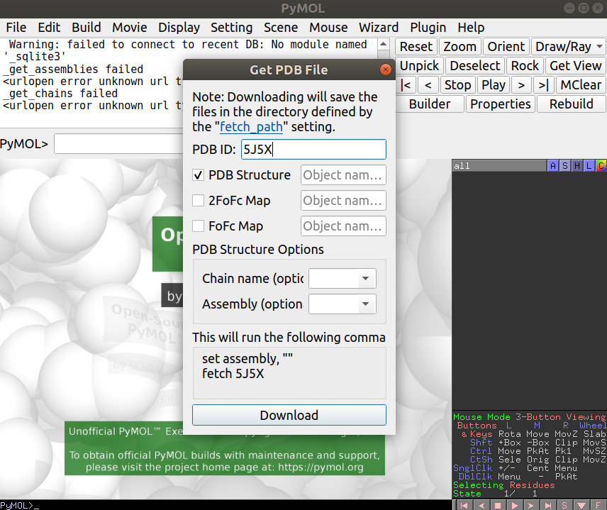
Open Pymol and load up the 5J5X structure. You can do this by going to File -> Get PDB and typing in the PDB id code you are interested in:

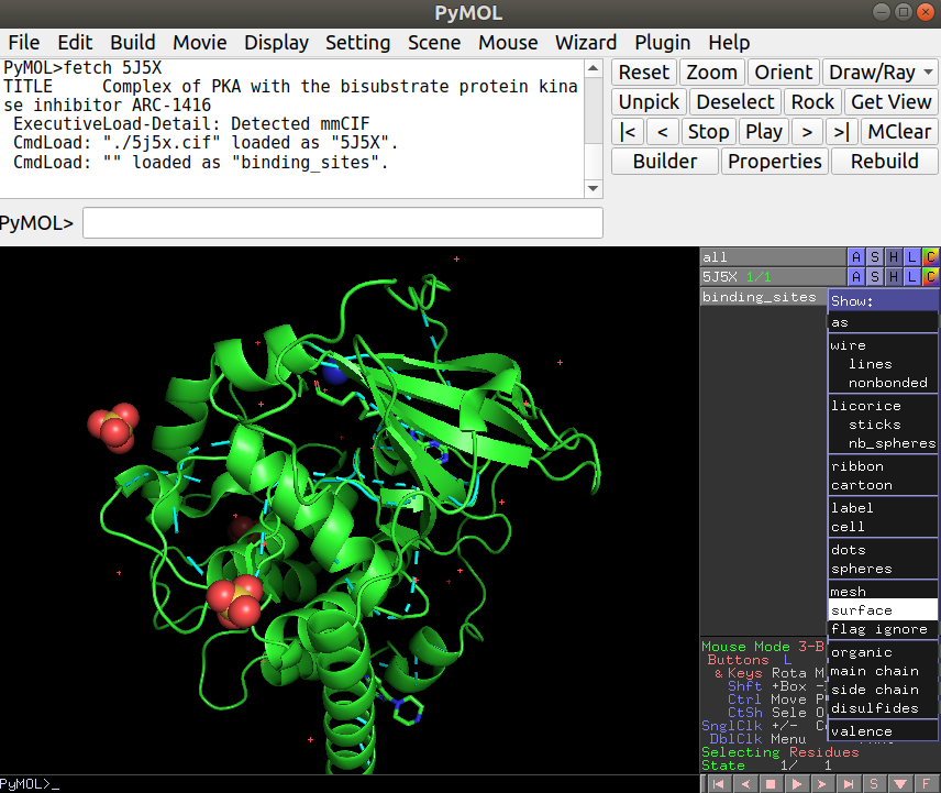
After loading this, you can now load the binding site PDB file you have created in R under File -> Open… and navigate to the appropriate file (“binding_sites.pdb”). Once you have this loaded you will see a thin line representing the binding site residues that you can now show as a surface representation by clicking in S (for Show) -> surface, just in the binding_sites object:

Instead of getting all binding sites residues we might be interested in finding the interface residues just for specific regions of the structure. For that we can first select the indices we want to use with the atom.select() function and then use those in the binding.site() function.

# Get just the interface residues between A and B
#Define the indices of chain A and chain B with atom.select
ainds <- atom.select(pdb, chain="A")
binds <- atom.select(pdb, chain="B")

# Define the binding sites using these indices
bs <- binding.site(pdb, a.inds = ainds, b.inds = binds)

# Write pdb to file as before
bs.pdb<-trim.pdb(pdb, inds = bs$inds)
write.pdb(bs.pdb, file = "binding_sites.pdb")

Pocket prediction algorithms

Small molecule binding sites are a specific subset of protein binding regions that are of particular interest for the development of novel drug therapies. These binding sites are often characterized as cavities with specific ligand binding residues that tend to be highly conserved and highly constrained to be at the same positions in homologous pockets. The prediction of pockets and the ligand binding residues is an important and well developed area of structural bioinformatics.

There are several different algorithms that use the 3D representation to predict pockets. One commonly used approach is to place the structure in a grid and each grid point is then scored based on criteria such as the distances from each point to the protein along different directions as well as physical chemical properties of the region or conservation properties of nearby residues. Selected points in the grid can then be clustered to find larger regions that may have properties that make them good pockets. After scoring and filtering relevant clusters, these can then be used to find binding sites.

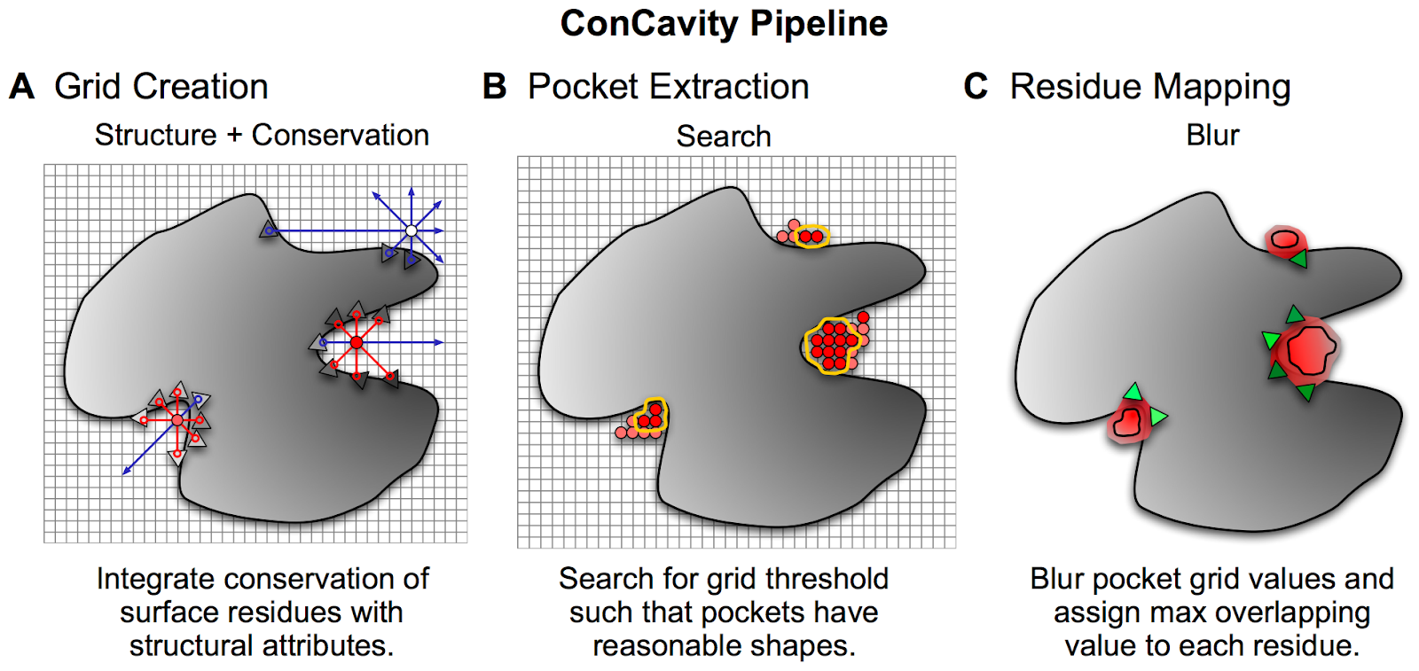
Example of a pocket and ligand binding site prediction method - From Capra et al. PLOS Comp Bio 2009 https://journals.plos.org/ploscompbiol/article?id=10.1371/journal.pcbi.1000585

Bio3D does not have in-built functions to perform pocket detection and we will not cover this further in this course. For those that may be interested in extending further their knowledge in this area, there are several command line tools that can be installed and used via the cluster/terminal. One example is fpocket which is easy to install and use. Pocket prediction and small molecule docking are covered in the Bioinformatics Concept Course for those interested in expanding their knowledge of bioinformatics.