Metagenomics II#
General information#
In this practical session, we will explore approaches and concepts for comparing the differences between samples, in line with the content of the second lecture.
More specifically, we will:
Compare differences between samples using beta-diversity indices
Visualise compositional differences in samples using Principle Components Analysis (PCA) and Principle Coordinates Analysis (PCoA)
Assess the distribution of species across samples using differential abundance testing
Learn how to apply a random forest model
Resources#
Exercises within the Metagenomics II section require the use of the R-Studio on cousteau: http://cousteau-rstudio.ethz.ch/
Dataset#
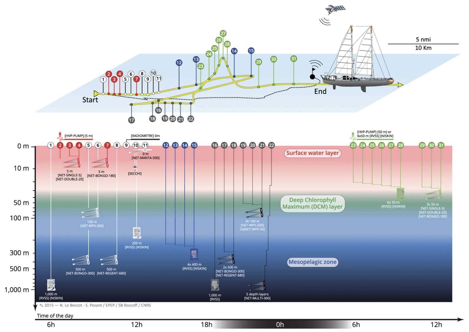
For this session, we will use an OTU dataset generated from microbial communities sampled at 68 locations across the world’s oceans during the Tara Ocean expedition in 2009 - 2013. At each of the locations, samples were collected at multiple depths, including the surface (SRF), deep-chlorophyll maximum (DCM) and mesopelagic (MES). These depths are typical of ocean sampling campaigns as they capture the vertical structuring of microbial communities in the upper ocean. To clarify what we refer to with the different depth layers:
SRF: top 5 m of the ocean
DCM: the depth at which chlorophyll a concentrations peak below the surface layer (often between 20 - 40 m)
MES: the layer in the ocean that separates the sunlit surface waters from the dark, deep waters (sometimes refered to as twilight zone)

The dataset that we will use in this session is a subsampled version of the much larger global dataset, which was published by Sunagawa et al., (2015) in Science.
load(url("https://sunagawalab.ethz.ch/share/teaching_materials/MGII_TO_data.Rdata"))
This will load two dataframes:
TO_otu_counts, contains an OTU taxonomic profileTO_otu_meta, contains information on the depth layer that each sample was collected
Taxonomic profile
The TO_otu_counts is a profile of the OTUs (‘species’) identified across 125 samples collected from three different depth layers of the ocean. The depth layer information is visible in the sample names (column names).
The abundances of the OTUs are expressed as raw counts.
Visualise the first few rows and columns of the profile (TO_otu_counts[1:3,1:3]):
        TARA_058_DCM    TARA_064_DCM    TARA_065_DCM
OTU_1   3413            6517            8856
OTU_2   994             1668            1553
OTU_4   380             972             1308
Metadata
The TO_otu_meta contains information to connect the samples to the depth layer from which they were collected.
Visualise the first few rows and columns of the metadata (TO_otu_meta[1:3,1:3])
Sample_name     Sample_station  Depth_layer
TARA_155_DCM    TARA_155        DCM
TARA_158_DCM    TARA_158        DCM
TARA_168_DCM    TARA_168        DCM