Session 1.8. Metagenomics analyses#
Technical advances in sequencing technologies in recent decades have allowed detailed investigation of complex microbial communities without the need for cultivation. Sequencing of microbial DNA extracted directly from environmental or host-associated samples have provided key information on microbial community composition. These studies have also allowed gene-level characterization of microbiomes as the first step to understanding the communities’ functional potential. Furthermore, algorithmic improvements, as well as increased availability of computational resources, make it now possible to reconstruct whole genomes from metagenomic samples (metagenome-assembled genomes (MAGs)). Here we describe building Metagenomic Assembly as well as building Gene Catalogs and MAGs from metagenomic data.
A lot of this tutorial is derived from:
Learning Goal#
The goal of this session is to understand the primary analysis steps required for the analysis of sequencing data, taxonomic and gene profiling, and the reconstruction of MAGs and execute the analysis pipeline on a controlled small dataset.
Input Data#
Raw sequencing data is usually encoded in the FASTQ format which combines sequence information with values that describe the quality of every single base.
The FASTQ files serve as input for our pipeline. There are always 2 files per sample, one for the R1 reads and one for the R2 reads. You can find the FASTQ files corresponding to 2 samples (use the Terminal, not the R Console):
# Create a working directory and copy the raw reads files
mkdir metagenome_analysis
cp /nfs/course/course_home/smiravet/reads/*.fq.gz .
Exercises#
Use linux commands to access one of the files and have a look to its content. Can you describe what are the different parts of the content?
Use linux commands to access all files and count the number of sequences in each. How would you count sequences in a FASTQ file?
Hints:
you may want to check the grep and wc linux command in Google or in the linux cheatsheet provided in the first session.
tar.gz files are compressed, you can read/parse them without decompressing using zcat and zgrep, respectively. Do the number matches for R1 and R2 files?
Data preprocessing#
We will NOT be running this initial steps as you are working with controlled synthetic generated data but this is a step required to perform with actual data.
Sequence Adapter Removal#
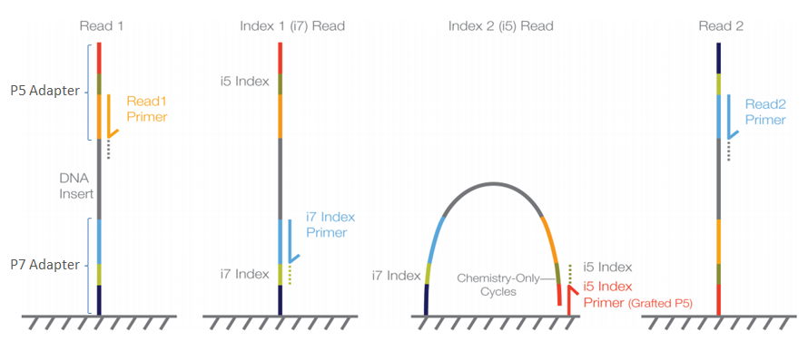
The adapter sequences contain the sequencing primer binding sites, index sequences, and sequences that allow flow-cell binding.

These primers need to be removed prior to analysis. There are two main reasons for that:
The sequence corresponding to the adapter may interfer the quantification of actual genomic DNA with similar sequences
The primers need to be detected to ensure that all sequences analyzed have been properly processed
For that purpose we use tools such as cutadapt or bbduk (from BBTools). These tools take the primer sequences and the FASTQ files as input and removes the primers that are in most cases at the beginning of the reads.
Command example:
bbduk.sh -Xmx1G usejni=t in=samp_R1.fq.gz in2=samp_R2.fq.gz \
out=samp_trimmed_R1.fq.gz out2=samp_trimmed_R2.fq.gz \
outm=samp_adapter_matched.fq.gz outs=samp_adapter_s.fq.gz  \
refstats=samp.adapter_trim.stats statscolumns=5 overwrite=t ref=adapters.fa \
ktrim=r k=23 mink=11 hdist=1 2>> preprocessing.log
Quality Control#
Sequencers have massively improved in terms of throughput and quality in the recent years. However they still produce erroneous bases. These appear usually at the end of the sequences but it can also happen that entire cycles lead to low quality bases. Then all reads have a lower quality at a specific position.
In order to remove sequences with bad quality and to remove low quality tails of otherwise good sequences we can use bbduk again
bbduk.sh -Xmx1G usejni=t in=samp_trimmed_R1.fq.gz in2=samp_trimmed_R2.fq.gz  \
out1=samp_clean_R1.fq.gz out2=samp_clean_R2.fq.gz \
outm=samp_qc_failed.fq.gz outs=samp_s.fq.gz minlength=45 \
qtrim=rl maq=20 maxns=1  stats=samp_qc.stats statscolumns=5 trimq=14 2>> qc.log
Taxonomic profiling#
Taxonomic profiling of complex microbial communities is an essential first step in the investigation of relationship between community composition and environmental and/or health factors. The most common approach to community profiling is amplification and classificaton the 16S rRNA gene. However, recently shotgun metagenomic sequencing has started to replace the amplicon based approaches, as it provides higher resolution information about the microbial community, and resolves some of the biases associated with 16S approach. A number of software tools have been developed to taxonomically profile metagenomic samples.
Here we’re going to use of mOTUs for taxonomic profiling (more information in lecture next week). This bioinformatics tool determines the composition of metagenomic samples using 10 single copy phylogenetic marker genes and an extensive database consisting of reference genomes, metagenomes and metagenome assembled genomes from 23 different environments. To run a basic mOTUs search:
# To use tools in the server we first need to upload them using the module load function
ml motus

# Create a folder for the results and run motus
mkdir motus_profiles

motus profile -f samp_R1.fq.gz -r samp_R2.fq.gz -n taxonomic_search -o motus_profiles/taxonomic_search.motus -k mOTU -c

# Remove the first two rows of the output file
tail -n+3 motus_profiles/taxonomic_search.motus > motus_profiles/taxonomic_search_headerless.motus

# Show the most abundant
sort -t$'\t' -k2 -rn motus_profiles/taxonomic_search_headerless.motus | head -n 10
Exercises#
What is -k defining?
Inspect the output file generated, what does this include?
Can you discuss on potential advantages of using single-copy genes to measure abundance over considering 16S rRNAs?
What is -k defining?
Can you make a plot with the taxonomic_search_headerless.motus
Reminder#
An operational taxonomic unit (OTU) is considered as the basic unit used in numerical taxonomy. These units may refer to an individual, species, genus, or class. OTUs are analytical units used in microbial ecology.
Metagenomic assembly#
We use metaSPAdes to assembly MAGs. This bioinformatics tool is part of the SPAdes assembly toolkit. Following the assembly, we generate some assembly statistics using assembly-stats, and filter out contigs that are < 1 kbp in length. The script we use for scaffold filtering can be found here: scaffold_filter.py. It is also included in the test dataset for this section
ml SPAdes
mkdir metag_assembly
metaspades.py -t 4 -m 10 --only-assembler --pe1-1 samp_R1.fq.gz --pe1-2 samp_R2.fq.gz -o metag_assembly/metag
Exercises#
What are -t and -m options doing?
Inspect the output file generated, what does this include?
The scaffolds.fasta include the assembled sequences in fasta format, how many?
Notes#
Computational resources needed for metagenomic assembly will vary significantly between datasets. In general, metagenomic assembly requires a lot of memory (usually > 100 Gb). You can use multiple threads (16-32) to speed up the assembly. Because test data set provided is very small, merging of the pair-end R1 and R2 reads was not necessary, but in real-case scenarios this is a step that can help to reduce the time/computer cost.
Filtering and evaluations of contigs#
Contigs produces can be too short to perform posterior analysis steps. Thus, we filter out contigs that are < 1 kbp in length. We will run a custom script written in python for this task:
# Copy the script
cp /nfs/course/course_home/smiravet/scaffolds_filter.py .

# Change directory and run script
cd metag_assembly

python ../scaffolds_filter.py metag scaffolds metag/scaffolds.fasta metag META

# Output is stored in out metag folder, check the output there
cd metag
Options:
metag - Sample name
scaffolds - Sequence type (can be contigs, scaffolds or transcripts)
metag_assembly/scaffolds.fasta - Input assembly to filter
metag - Prefix for the output file
META - Type of assembly (META for metagenomics or ISO for isolate genomes)
This step will split the sequences by scaffold nucleotide lenght in our metag folder in three files: metag.scaffolds.min0.fasta, metag.scaffolds.min500.fasta, metag.scaffolds.min1000.fasta
Exercises#
How many sequences remain after filtering the scaffolds.fasta file with each length threshold?
Assembly statistics#
General statistics of the sequences generated can be explored using:
assembly_stats metag.scaffolds.min500.fasta > metag.assembly.stats
Exercises#
What has assembly_stats written?
N50 statistic defines assembly quality in terms of contiguity. Given a set of contigs, the N50 is defined as the sequence length of the shortest contig at 50% of the total assembly length.
Given a set of contigs, each with its own length, the L50 is defined as count of smallest number of contigs whose length sum makes up half of genome size. From the example above the L50=3.
Gene catalogs#
The metagenomic scaffolds generated can now be used to build and/or profile Gene Catalogs. This catalog generation and profiling (i.e. gene abundance estimation) can provide insights into the community’s structure, diversity and functional potential. This analysis could also identify relationships between genetic composition and environmental factors, as well as disease associations when exploring clinical-derived samples.
Integrated catalogs of reference genes have been generated for many ecosystems (e.g. ocean, human gut, and many others) and might be a good starting point for the analysis.
Gene calling#
We use prodigal to extract protein-coding genes from metagenomic assemblies. Prodigal has different gene prediction modes with single genome mode as default. To run prodigal on metagenomic data, we add the -p meta option. This will produce a fasta file with amino acid sequences (.faa), nucleotide sequences (.fna) for each gene, as well as an annotation file (.gff).
cd ../../

ml prodigal

mkdir gene_calling

prodigal -a gene_calling/metag.faa -d gene_calling/metag.fna -f gff -o gene_calling/metag.gff -c -q -p meta -i metag_assembly/metag/metag.scaffolds.min500.fasta
Exercises#
What is doing the -c option?
What is the difference between .faa and .fna files? And .gff?
How many sequences there are in those files?
Gene de-replication.#
At this point gene-nucleotide sequences from all samples are concatenated together and duplicated sequences are removed from the catalog. For this, genes are clustered at 95% identity and 90% coverage of the shorter gene using CD-HIT. The longest gene sequence from each cluster is then used as a reference sequence for this gene.
ml CD-HIT

mkdir gene_catalog

cp gene_calling/metag.fna gene_catalog/gene_catalog_all.fna
cp gene_calling/metag.faa gene_catalog/gene_catalog_all.faa

cd gene_catalog

mkdir cdhit9590

cd-hit-est -i gene_catalog_all.fna -o cdhit9590/gene_catalog_cdhit9590.fasta -c 0.95 -T 64 -M 0 -G 0 -aS 0.9 -g 1 -r 1 -d 0
The fasta file generated by CD-HIT will contain a representative nucleotide sequence for each gene cluster.
To extract protein sequences for each gene in the catalog, we first extract all the sequence identifiers from the CD-HIT output file and use seqtk subseq command to extract these sequences from gene_catalog_all.faa. This file can be then used for downstream analysis, for example to extract KEGG annotations.
ml seqtk

grep "^>" cdhit9590/gene_catalog_cdhit9590.fasta | \

cut -f 2 -d ">" | cut -f 1 -d " " > cdhit9590/cdhit9590.headers

seqtk subseq gene_catalog_all.faa cdhit9590/cdhit9590.headers > cdhit9590/gene_catalog_cdhit9590.faa
Exercises#
What is cut doing?
Note#
These steps are highly dependent on the total number of sequences and different species found in a raw sequencing read file, as we are working with a limited dataset, this step is not performing quite well.
Gene Catalog Profiling#
This protocol allows quantification of genes in a gene catalog for each metagenomic sample (makes sense to be run with >1 samples).
In the first step, sequencing reads are mapped back to the gene catalog using BWA aligner. Note that forward, reverse, singleton and merged reads are mapped separately and are then filtered and merged in a later step. We will just test the step with one of the samples.
Then, gene abundance can be step counts the number of reads aligned to each gene for each of the samples.
cd ..

ml BWA SAMtools

mkdir alignment

bwa index gene_catalog/cdhit9590/gene_catalog_cdhit9590.fasta

bwa mem -a -t 4 gene_catalog/cdhit9590/gene_catalog_cdhit9590.fasta ./samp_R1.fq.gz | samtools view -F 4 -h - > alignments/samp.r1.sam
Posterior steps can process these sam files to predict the abundance of specific genes in each sample by counting the number of reads aligned to each gene and compare between samples to extract functional information.
MAG reconstruction#
One of the greatest achievements in metagenomics is to be able to assemble individual microbial genomes from complex community samples. However, short-read assemblers fail to reconstruct complete genomes. For that reason, binning approaches have been developed to facilitate creation of Metagenome Assembled Genomes (MAGs).
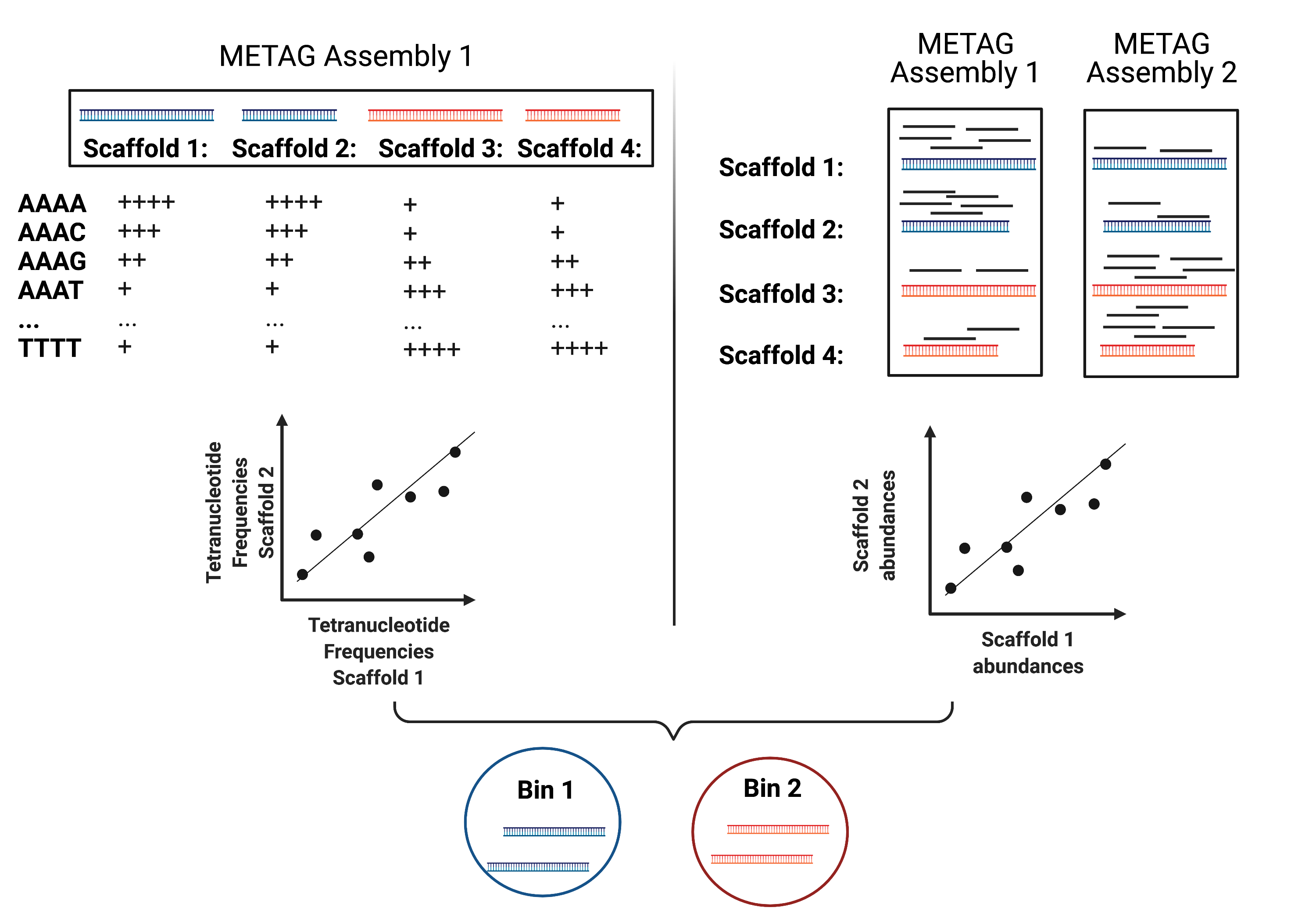
MAG reconstruction algorithms have to decipher which of the scaffolds generated during Metagenomic Assembly belong to the same organism (refered to as bin). While different binning approaches have been described, here we use MetaBAT2 for MAG reconstruction. As shown in the figure below, MetaBAT2 uses scaffolds’ tetranucleotide frequencies and abundances to group scaffolds into bins.

In this simplified example, the blue scaffolds show similar tetranucleotide frequencies and similar abundances and consequently end up binned together and separately from the red scaffolds.
MAG Building#
This workflow starts with size-filtered metaSPAdes assembled scaffolds (resulted from Metagenomic Assembly). Note that for MAG building we are using >= 1000 bp scaffolds.
1. All-to-all lignment: In this step, quality controlled reads for each of the metagenomic samples are mapped to each of the metagenomic assemblies using BWA. Here we use -a to allow mapping to secondary sites.
Working in our main directory metagenome_analysis
# Create BWA index for each assembly

ml BWA

bwa index metag_assembly/metag/metag.scaffolds.min1000.fasta

bwa mem -a -t 16 metag_assembly/metag/metag.scaffolds.min1000.fasta samp_R1.fq.gz \
    | samtools view -F 4 -bh - | samtools sort -O bam -@ 4 -m 4G > alignments/metag1_to_metag.1.bam

bwa mem -a -t 16 metag_assembly/metag/metag.scaffolds.min1000.fasta samp_R2.fq.gz \
    | samtools view -F 4 -bh - | samtools sort -O bam -@ 4 -m 4G > alignments/metag2_to_metag.2.bam

samtools merge alignments/metag_to_metag.bam alignments/metag1_to_metag.1.bam alignments/metag2_to_metag.2.bam
Note#
This is done with multiple samples, we will run the process with our two different R1 and R2 files, but it is just as an example. In actual data analyses we would do this iterating for every sample against every sample.
2. Within- and between-sample abundance correlation for each contig: MetaBAT2 provides jgi_summarize_bam_contig_depth script that allows quantification of within- and between-sample abundances for each scaffold. Here we generate an abundance (depth) file for each metagenomic assembly by providing the alignment files generated using this assembly. This depth file will be used by MetaBAT2 in the next step for scaffold binning.
ml MetaBAT

jgi_summarize_bam_contig_depths --outputDepth alignments/metag.depth alignments/metag_to_metag.bam
Exercises#
What does metag.depth file include?
Can you bring this file to R to visualize the depth of the largest contig?
# Transform the bam file to a pile-up depth
samtools depth alignments/metag_to_metag.bam > alignments/pileup.depth

# Filter for the largest scaffold (-w option in grep for exact match)
grep -w  "metag-scaffold_1" pileup.depth > metag-scaffold_1.depth
# Libraries
library(ggplot2)

# create data
t <- read.table(file = 'alignments/metag-scaffold_1.depth', sep='\t')

# Plot
ggplot(t, aes(x=V2, y=V3)) +
  geom_line()
3. Metagenomic Binning. Finally, we run MetaBAT2 to bin the metagenomic assemblies using depth files generated in the previous step.
mkdir mags

metabat2 -i metag_assembly/metag/metag.scaffolds.min1000.fasta -a alignments/metag.depth -o mags/metag --minContig 1500 --maxEdges 500 -x 1 --minClsSize 20000 --saveCls -v
Exercises#
How many contigs have we reconstructed?
4. Quality Control: After MAG reconstruction, it is important to estimate how well the binning perform. CheckM places each bin on a reference phylogenetic tree and evaluates genome quality by looking at a set of clade-specific marker genes. CheckM outputs completeness (estimation of fraction of genome present), contamination (percetange of foreign scaffolds), and strain heterogeneity (high strain heterogeneity would suggest that contamination is due to presence of closely related strains in your sample).
ml CheckM
checkm lineage_wf mags mags -x fa -f mags/checkm_summary.txt --tab_table
Exercises#
How do we interpret the checkm_summary table?
Again, these results have been obtained with a sample which is far from real data, in the following session we will be working with the Ocean Microbiome Database and you will have the opportunity to work with the completion and contamination values of the comprehensive MAG search done for ocean metagenomic samples.
Overview#

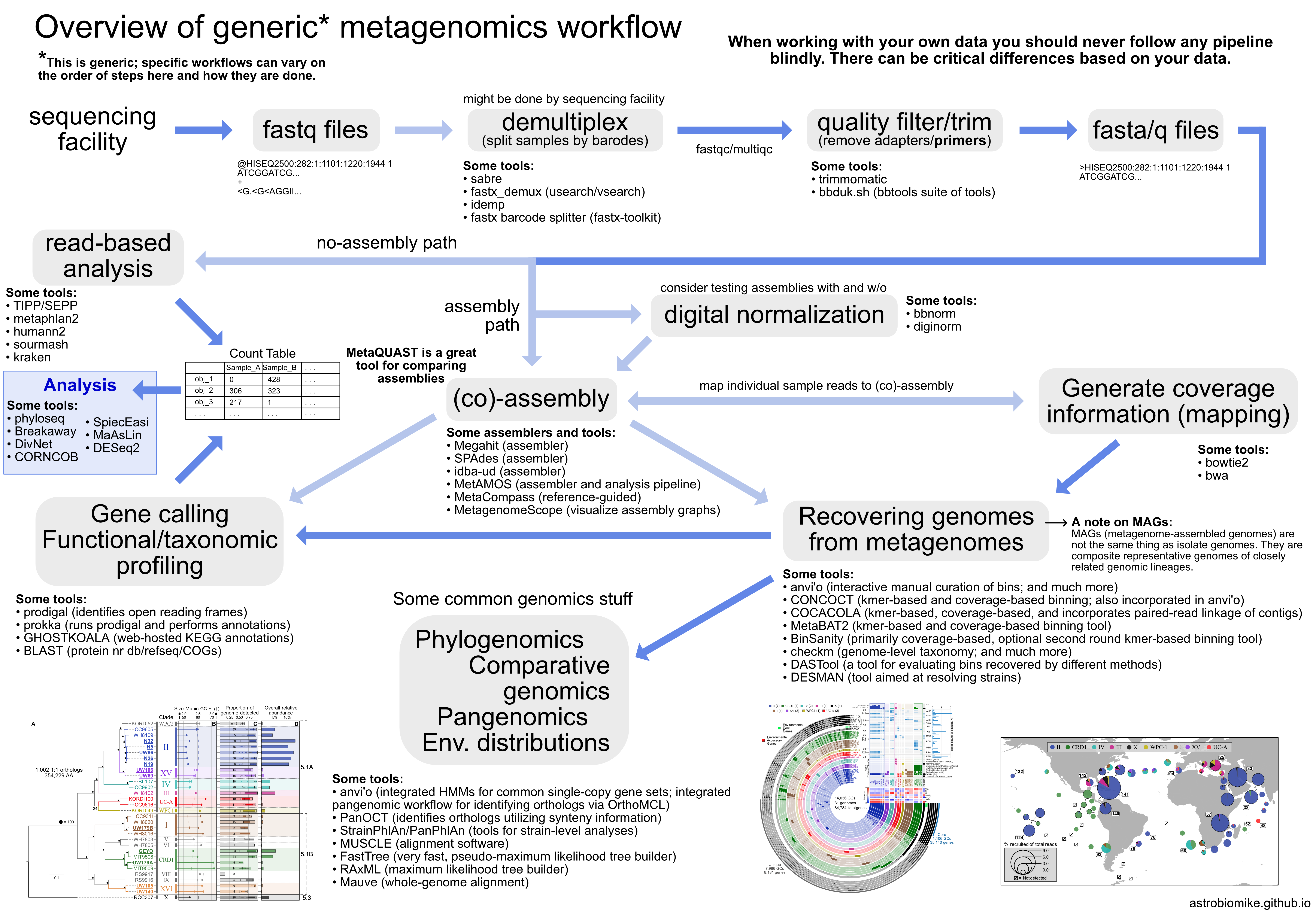
From Astrobiomike