Basic Concepts in Statistics#
In this brief course, we will look at statistics from the point of view of a researcher who is planning, or has collected data from an experiment and wants to draw conclusions from it that stand up to scrutiny. Before understanding the sort of tests we can perform on our data, we need to understand some of the basic properties of the data itself.
Simple Measures#
The arithmetic mean is the simplest measure of average that everyone is familiar with.
The median is the ‘middle value’ if all values were arranged in order.
Related to the median are quartiles and quantiles which tell you the value 25% or 75%, or an arbitrary percentage of the way through the data, if arranged in order.
The mode is the most frequent value(s).
Finally, the minimum and maximum are the lowest and highest values, covering the range of the data.
Variability#
Perhaps the most important factor in data analysis is variability. Biology is a very messy field of study with many sources of noise: from instruments used to take measurements, from the stochastic differences inherent in a population of cells, from barely controllable factors that change from experiment to experiment, and so on. Wherever possible we try to control for these, by taking repeat measurements, repeat samples and repeat experiments, as well as designing suitable controls that inform us what exactly is causing the observed differences in a treated sample.
The standard deviation is the most common measure of variability.
The formula above is for the sample standard deviation, which gives an unbiased estimate of variability. For the population measure, instead divide by N, which is accurate when you have all possible values. Otherwise use the sample measure, although even more accurate measures can be found for data that follows a particular distribution.
The variance is simply the standard deviation squared.
A useful measure of how far a particular value is from the mean is the standard or z-score.
The coefficient of variation is useful for comparing the spread of different sets of data and is calculated by dividing the standard deviation by the mean.
Properties of Data#
A set of data as a whole can have various properties that make it easier or more difficult to work with, and determine whether or not it might be suitable for a particular statistical test.
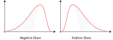
Data that is evenly spread about its mean, i.e.: the median is equal to or very close to the mean, is symmetrical.
If not, then we refer to the skew of the data. Positively skewed data has a long high tail and the median is lower than the mean. Negatively skewed data has a long low tail and the median is higher than the mean.

Data that could be any value (excepting the precision of your instruments) is continuous, whereas count data is discrete.
Certain types of count data, such as from short-read sequencing, might be compositional, i.e.: if the count of one item in the data goes up in a particular sample, the other counts must necessarily go down. This is much harder to work with!
Typical Distributions#
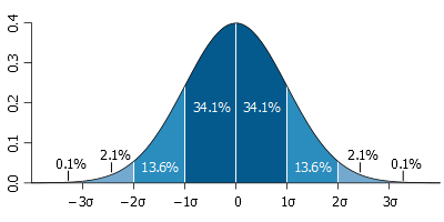
The most common and easiest data distribution to work with is the normal or gaussian distribution. It is continuous and symmetrical, with a relationship between mean and variance that results in 68% of the data with a z-score less than 1, 95% with a z-score less than 2, and 99.7% with a z-score less than 3.

Another related distribution that is the result of multiplying many random variables, is the log-normal distribution. This means that if you take the log of your data values, they will appear normally distributed.
Another common distribution is the Poisson, which describes the probability of a number of events occuring based on an occurence rate. It is discrete and asymmetrical, where both the mean and variance are equal to a single parameter, lambda.
Related to the poisson, the exponential distribution describes the time between events in a Poisson process. It is continuous and asymmetrical.
The binomial distribution describes the probability of a number of successes in a number of tests, each of which is equally likely to succeed. It is discrete.
The related hypergeometric distribution describes the probability of drawing a number of objects from a collection in a number of draws, where the objects are not replaced as they are drawn. It is also discrete.
Useful R Functions#
mean and median return their respective values, but perhaps more useful is summary on a vector of numbers, which returns almost all the simple measures listed above.
range returns the minimum and maximum values alone.
There is no built-in function for mode, but table will perform a frequency count of values, and sort will arrange them from lowest to highest frequency.
quantile by default returns quartiles, but you can give an argument to return any quantiles you like.
sd and var return the sample standard deviation and variance respectively.
To understand the properties of your data, it’s usually a good idea to plot it. A histogram is a good way to understand a distribution, and R offers the function hist.
# Plot a histogram
data(iris)
h = hist(iris[,1])
h = hist(iris[,1],breaks=20)
An alternative is to consider the cumulative distribution. R has the function ecdf, or slightly more flexible is Ecdf in the package Hmisc.
# ecdf
e = ecdf(iris[,1])
plot(e)

# Ecdf
E = Ecdf(iris[,1])
E = Ecdf(iris[,1],what='f')
If you want to generate data that conforms to a particular distribution, there are consistently named functions for each of the distributions mentioned above. Taking the normal as example, dnorm generates the density function, pnorm generates the distribution function, qnorm generates the quantile distribution and rnorm chooses random values from the distribution. You can use the d, p, q and r prefixes with pois, exp, binom and hyper for those distributions.
# Normal examples
plot(-30:30/10,dnorm(-30:30/10))
plot(-30:30/10,pnorm(-30:30/10))
plot(1:99/100,qnorm(1:99/100))
hist(rnorm(1000))
Exercises#
Load the LakeHuron data set and determine for yourself what properties the data has, and whether it looks like a particular distribution or not.
Load the treering data set and repeat the exercise.