Protein interfaces and structural similarity
General information
Main objective
In this lecture we will study different types of protein interfaces and binding pockets, how they can be identified and predicted from protein structures. We will also discuss protein structural similarity and its relationship with sequence similarly. We will learn different approaches and metrics to identify structurally related proteins and how to perform structural alignments computationally.
Learning objectives
Students understand key differences between different types of protein interfaces
Students understand the differences and relationship between protein sequence and structural similarly
Students gain proficiency in finding interface residues within structures and calculating structural similarity with R
Resources
This section requires the use of the R Studio: http://cousteau-rstudio.ethz.ch We will also need Pymol in order to visualize some of the results: https://pymol.org/2/
Video
This section has a complementary video:
Protein pockets and interaction interfaces
Protein molecules don’t work in isolation and will instead interact with other proteins, DNA/RNA or small molecules in order to be able to perform their functions. Therefore, in order to understand and study protein function we need to understand as well how they interact with other molecules. In addition, these interaction sites are used to design drugs that can alter protein behavior which is essential for rational design of therapies but also important for the development of tool compounds that are used to study biological systems .
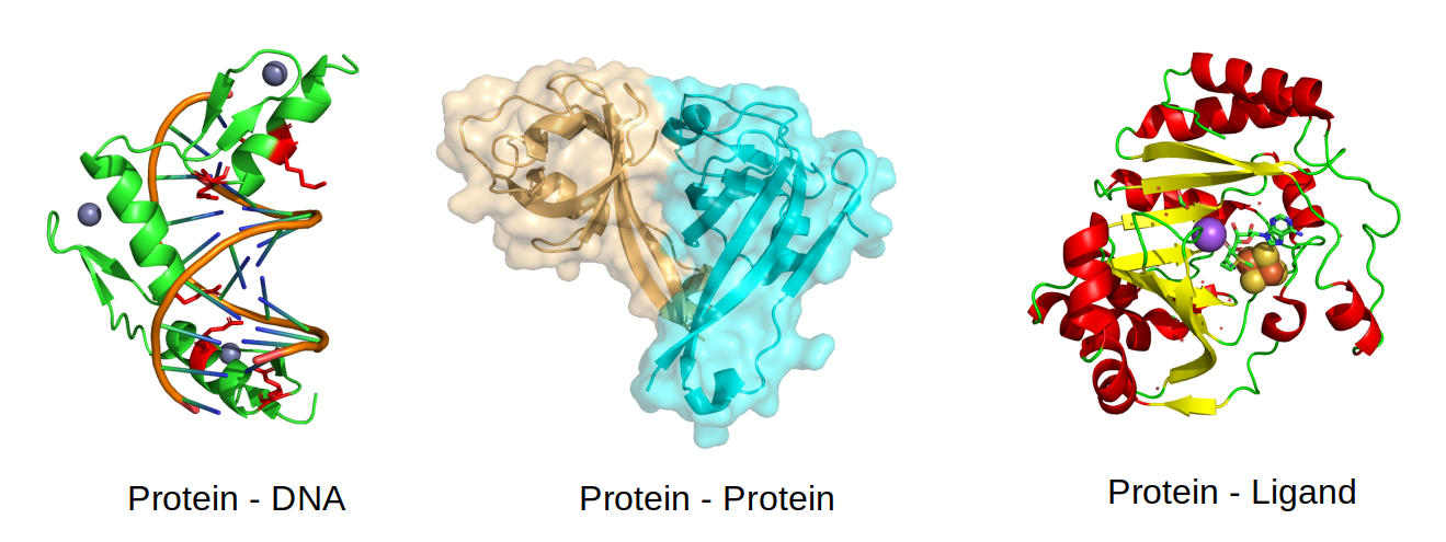
Not all protein interaction sites are the same and they can be broadly split into protein-protein interactions, protein-DNA/RNA interactions and binding sites for small molecules. Protein-protein interactions can be also classified according to properties of the interaction such as the size of the interface, the affinity or strength of interaction and its lifetime which could be transient or permanent. The interaction with small-molecules is most often occurring within well defined pockets within a protein structure, while interactions with other proteins or DNA/RNA occurs in more “flat” surfaces that are more espoused to the surface. Such binding sites within proteins are also usually classified in different types such a binding site for the substrate of the enzyme (i.e. an active site) or a binding site distal to the active site that can module enzyme function through a change in conformation (i.e. allosteric site).
The interactions are stabilized by non-covalent interactions of different types (e.g. hydrogen bonds and ionic interactions) and by the hydrophobic effect, whereby the interaction tends to be stabilized when hydrophobic amino-acids are forming an interface instead of being exposed to the solvent. Not all residues at an interface contribute equally to complex formation and understanding which residues are important and why, is key to study for example the impact of mutations. Critical interaction residues tend to be more conserved over the course of evolution. For example, the protein-DNA illustrated below is stabilized by positively charged residues in the protein (in red) with negatively charged residues in the DNA. Large protein-protein interfaces such as the one shown below are most often stabilized by buried hydrophobic amino-acids and some of the specificity can come from complementary shape. The interactions between proteins and small molecules often happens at pockets, as the one shown below, where a few key residues determine the interaction and consequent catalysis.
Identifying or predicting protein interaction sites
If we already have a protein structure bound to a protein or small molecule, we can identify the interaction surface by simply calculating the distances between atoms and then selecting residues that are close in space to the binding molecule. Alternatively, we can also calculate surface accessibility of the protein residues in the presence or absence of the binding molecule. The interface residues would be those that increase the most in their surface accessibility.
When we don’t already have a structure of binding site we can still try to predict if there are regions within the structure that may be interaction surfaces. The following properties are often used by computational methods that look for contiguous regions (i.e. patches) at the surface that could be such interface regions: * Amino acid types and their physicochemical properties - patches of amino-acids that are hydrophobic are for example more likely to be an interface region * Evolutionary properties - Critical interface residues are more conserved and may also co-evolve with the residues in the putative interacting protein * Surface accessibility and shape - Interaction regions need to be accessible and may have specific shape characteristics. * Homology with other structures - if the structure of interest has an homologous structure bound to an interacting partner the same regions within the structure of interest can be predicted as an interface region.
If you want to study these topics at a more advanced level you can read a review article that goes into more details on computational methods to predict interface residues (Xue et al. FEBS letter 2016).
Identifying interaction sites with Bio3D
Let’s start by using Bio3D to identify binding residues with the binding.site() function and the same protein kinase structure (5J5X) as before. This function can find residues between different entities (e.g. chains or small molecules) using a distance based cutoff that is set to 5 angstroms as default. When no indices are given the function will find all binding sites by default.
# Use the bio3d library
library(bio3d)

# Fetch the PDB structure with a PDB code id
pdb <- read.pdb("5J5X")

# Find all interface residues
bs <- binding.site(pdb)
The object bs will now hold the binding site information which includes the indices (bs$inds), residues names (bs$resnames) and number (bs$resno). The indices can be used in other functions of the Bio3D package such as the trim.pdb() function. To visualize the binding sites we can create a PDB file that has these binding residues and overlay them on top of the original structure for comparison.
# Extract binding atoms and print a new PDB with this
bs.pdb <- trim.pdb(pdb, inds = bs$inds)
write.pdb(bs.pdb, file = "binding_sites.pdb")
In order to visualize the binding sites we will use Pymol. You will need to download the file you have generated by selecting the file within the RStudio Workbench Files tab, then selecting More and Export. In this way you can move files from the Workbench to your local computer for viewing.
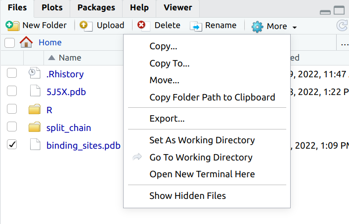
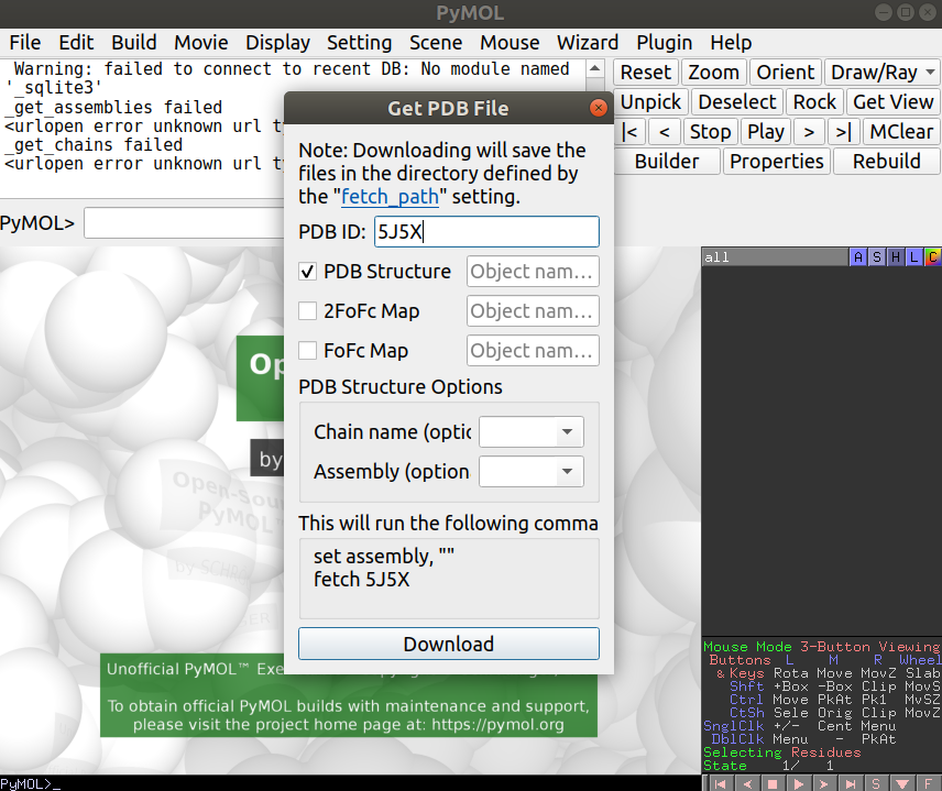
Open Pymol and load up the 5J5X structure. You can do this by going to File -> Get PDB and typing in the PDB id code you are interested in:
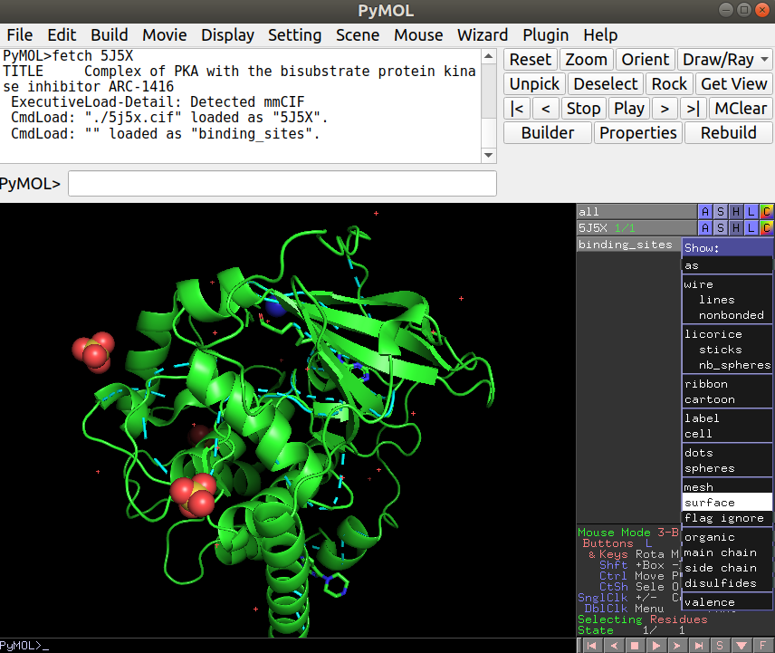
After loading this, you can now load the binding site PDB file you have created in R under File -> Open… and navigate to the appropriate file (“binding_sites.pdb”). Once you have this loaded you will see a thin line representing the binding site residues that you can now show as a surface representation by clicking in S (for Show) -> surface, just in the binding_sites object:
Instead of getting all binding sites residues we might be interested in finding the interface residues just for specific regions of the structure. For that we can first select the indices we want to use with the atom.select() function and then use those in the binding.site() function.
# Get just the interface residues between A and B
#Define the indices of chain A and chain B with atom.select
ainds <- atom.select(pdb, chain="A")
binds <- atom.select(pdb, chain="B")

# Define the binding sites using these indices
bs <- binding.site(pdb, a.inds = ainds, b.inds = binds)

# Write pdb to file as before
bs.pdb<-trim.pdb(pdb, inds = bs$inds)
write.pdb(bs.pdb, file = "binding_sites.pdb")
Pocket prediction algorithms
Small molecule binding sites are a specific subset of protein binding regions that are of particular interest for the development of novel drug therapies. These binding sites are often characterized as cavities with specific ligand binding residues that tend to be highly conserved and highly constrained to be at the same positions in homologous pockets. The prediction of pockets and the ligand binding residues is an important and well developed area of structural bioinformatics.
There are several different algorithms that use the 3D representation to predict pockets. One commonly used approach is to place the structure in a grid and each grid point is then scored based on criteria such as the distances from each point to the protein along different directions as well as physical chemical properties of the region or conservation properties of nearby residues. Selected points in the grid can then be clustered to find larger regions that may have properties that make them good pockets. After scoring and filtering relevant clusters, these can then be used to find binding sites.
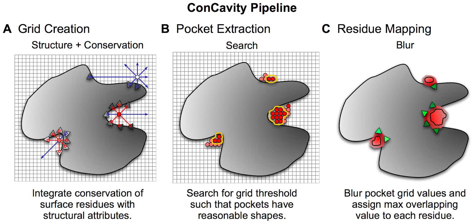
Example of a pocket and ligand binding site prediction method - From Capra et al. PLOS Comp Bio 2009 https://journals.plos.org/ploscompbiol/article?id=10.1371/journal.pcbi.1000585
Bio3D does not have in-built functions to perform pocket detection and we will not cover this further in this course. For those that may be interested in extending further their knowledge in this area, there are several command line tools that can be installed and used via the cluster/terminal. One example is fpocket which is easy to install and use. Pocket prediction and small molecule docking are covered in the Bioinformatics Concept Course for those interested in expanding their knowledge of bioinformatics.
Protein structural similarity
Proteins can be aligned by their structure instead of by their sequence. In protein structural alignment the objective is to find commonalities in the three dimensional structure which may or not relate to similarity of the primary sequence. There are many different algorithms that have been developed to perform structural alignments and also many different measurements to try to quantify the degree of structural similarity between structures. One idea that has been commonly used is to try to move and rotate one of the structures in such a way that it minimizes the distance between potentially equivalent atoms (see schematic of figure below). To achieve this, there needs to be a measurement of similarity that can be optimized and a very efficient way to search through the possible rotations and movements of the structures.
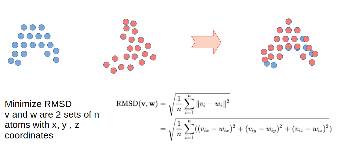
A very commonly used metric of structural similarity is called the root-mean-square deviation of atomic positions or RMSD. Given a set of two superimposed structures, RMSD is a measure of the average distance between atoms expressed in units of length, most commonly in Ångström (Å or 10−10m). RMSD can be calculated for any set of pairs of atoms depending on the application and two common sets would be all atoms or just the C-alpha atoms. There are many other algorithms to align structures that make use of other ideas such as comparing overall shapes or comparing sets of structural elements.
The similarity of protein structures can be used to predict protein function by structural homology. For example, there may be a similar pocket in both proteins which would help annotate an enzymatic activity that was unknown. Proteins with highly identical sequences will almost always have very identical structures. However, it is possible for proteins to have highly identical structures with very divergent sequences.
The Bio3D library can be used to perform and score structural alignments. In order to select a set of structures to align we can also use a Blast search to find structures that have sequences that are similar to the sequence of the kinase structure we have been analyzing (5J5X).
# Use the bio3d library
library(bio3d)

# Fetch the PDB structure with a PDB code id
pdb <- read.pdb("5J5X")

# Create a new PDB object just with A chain with the kinase domain
apdb <- trim.pdb(pdb, chain="A")

# Retrieving the protein sequence
seq <- pdbseq(apdb)

# Use Blast to query the PDB for structures of related sequences
blastResult <- blast.pdb(seq)
top.hits <- plot.blast(blastResult, cutoff=100)
The blast.pdb() function uses the sequence to find structures in the PDB that have related sequences. This information is stored in the blastResult object, which can be inspected using the plot.blast() function. This also returns a list of hits that can be stored for further queries. In this case, the hits were stored in the object top.hits.
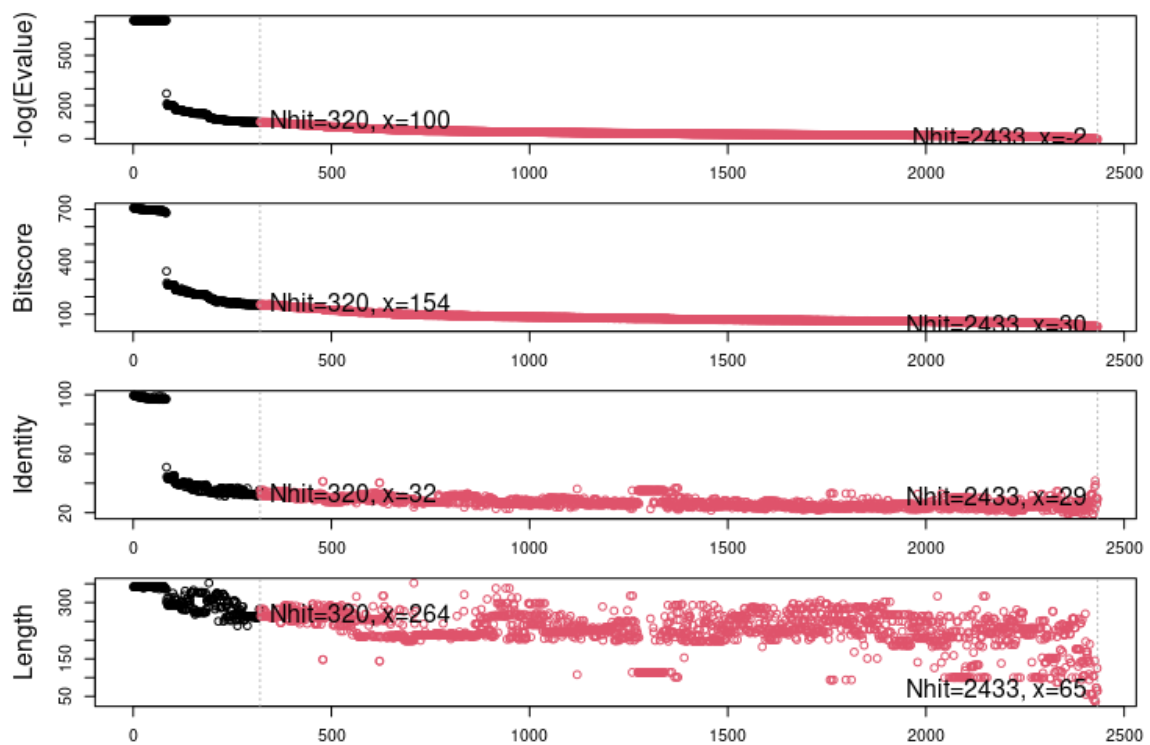
The plot above shows the visual representation of the blast results, indicating a number of highly identical sequences followed by a larger number of less related sequences. For the structural alignment we will focus on the structures having the top 10 most similar sequences based on this blast search. The structural alignment function in Bio3D takes advantage of having a multiple sequence alignment which is done via muscle.
# Get the PDBs for the top 10 blast hits split by chain. These will be stored in ./split_chain/. My_pdbs will hold the list of downloaded PDBs. notice that we used get.pdb() instead of read.pdb()
my_pdbs<-get.pdb(top.hits$hits[1:10], split = TRUE)

#Shortcut
my_pdbs<-get.pdb(c("7VRV_A","7JWB_A","7BYR_A","6ZP1_A","7EJ4_A","7FCD_A","7OAN_A","7WCD_C","7CAI_A","7A25_A"), split = TRUE)

# pdbaln() takes a list of PDBs to aln using MUSCLE
aln_pdbs <- pdbaln(my_pdbs)

# Structural alignment and output all fitted structures to outpath
xyz <- pdbfit(aln_pdbs, outpath="fitted")
The function pdbfit() is the function that performs the structural alignment and it is based on the minimization of the RMSD using the Kabsch algorithm. It takes advantage of the sequence alignment to have an idea of which residues are likely to be the same in different structures. The outcome of the structural alignment is a set of new PDB files that are stored in the folder “./fitted/”. These PDB files have each of the 10 structures all represented in the coordinates of the aligned structures. The pdbfit() function also returns the coordinate values for the aligned atoms, which are collapsed into a matrix format and stored in xyz. This object with coordinates can then be used in different ways to calculate and display measurements of similarity.
# Calculate RMSD
rd <- rmsd(xyz)
rd
2F7E_E 3AGM_A 3MVJ_A 6C0U_A 5VI9_A 3NX8_A 3AGL_A 1CTP_E 4WB5_A 2C1A_A
2F7E_E  0.000  0.457  0.543  4.614  1.081  0.623  0.643  1.271  0.495  0.265
3AGM_A  0.457  0.000  0.711  4.644  0.924  0.818  0.713  1.124  0.724  0.440
3MVJ_A  0.543  0.711  0.000  4.715  1.316  0.577  0.679  1.510  0.431  0.574
6C0U_A  4.614  4.644  4.715  0.000  4.770  4.663  4.672  4.892  4.679  4.663
5VI9_A  1.081  0.924  1.316  4.770  0.000  1.273  1.362  0.581  1.276  1.007
3NX8_A  0.623  0.818  0.577  4.663  1.273  0.000  0.893  1.469  0.506  0.677
3AGL_A  0.643  0.713  0.679  4.672  1.362  0.893  0.000  1.577  0.750  0.665
1CTP_E  1.271  1.124  1.510  4.892  0.581  1.469  1.577  0.000  1.467  1.208
4WB5_A  0.495  0.724  0.431  4.679  1.276  0.506  0.750  1.467  0.000  0.510
2C1A_A  0.265  0.440  0.574  4.663  1.007  0.677  0.665  1.208  0.510  0.000
# Show the RMSD values for a specific pair
rd["5VI9_A","3NX8_A"]
1.273
Exercise 9.1
Calculate the largest, mean and median RMSD values (Tip - use na.rm = TRUE to exclude NAs)
max(rd, na.rm = TRUE)
4.892

mean(rd, na.rm = TRUE)
1.46904

median(rd, na.rm = TRUE)
0.784
We can see that overall the structures tend to be highly similar (RMSD <2A). This is expected since we selected structures that are highly related by sequence. However, there are also some exceptions that suggest that there may be different conformations adopted in the different structures. To get a more visual representation of the groups of structures that are more similar to each other we can perform a clustering analysis.
# Perform hierarchical clustering of the structural similarity using as a distance the RMSDs
hc.rd <- hclust(as.dist(rd))

# Plot the hc - see how different groups are formed
plot(hc.rd)

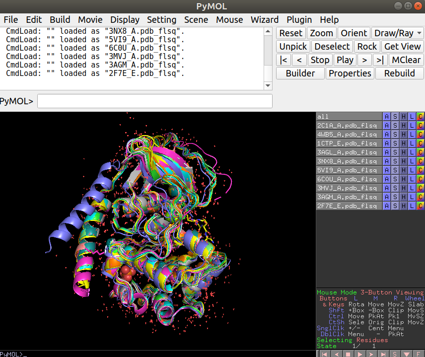
The plot above shows how the structures are grouping in terms of structural similarity. Based on these we can select some structures for visualization to better understand their differences. The superimposed structures can be found in the working directory under the folder “./fitted”. These can be downloaded to your local computer from the workbench as before and opened in Pymol together for visualization. For this you can open Pymol and simply select all the structures and drag them onto the Pymol window or through the menu select File -> Open and shift select all the structures that you want to see.
Exercise 9.2
Open the structures 6C0U_A together with any 2 other structures. What is visually different about 6C0U_A?
The N-terminal helix is in a very different location relative to the other structures
Advanced analysis - Bio3D has a set of functions that allows the user to generate a trajectory from interpolated structures that are based on a Principal Component Analysis (PCA). The following section explains how this is done and can be explored at a more advanced level.
Performing a PCA on the aligned atomic coordinates will identify the main axes of variation in the atomic coordinates. In essence, it will allow us to find the most striking differences in shape and also predict any arbitrary number of shapes along the path between these different shapes. This can be used as an hypothesis of potential dynamical behavior of the protein. The PCA on aligned atomics coordinates uses the pca.xyz() function.
# Performing PCA on the aligned structures
pca_data <- pca.xyz(xyz = xyz, rm.gaps = TRUE)

# Plot the results of PCA
plot(pca_data)
The plot below is a summary of the PCA analysis showing each of the structures represented in the lower dimension of the first 3 components. It also shows the proportion of variation in atomic coordinates that is explained by each component. These components and their degree of variation can be interpreted as possible structural dynamics.
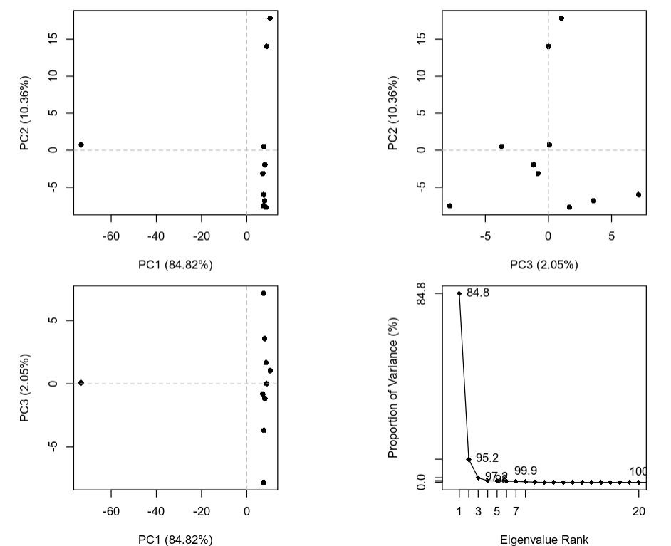
We can obtain information on the relative importance/score (PCA loadings) of each structure and each residue along these main predicted dynamical behaviors. The information for the structures is stored in pca_data$z and the equivalent for the residues in pca_data$au. For example to find the most variable residues along a specific principal component (dynamical behavior) we can plot it:
# Plot the degree of variability of each residue along PC1
plot.bio3d(pca_data$au[,1], ylab="PC1")
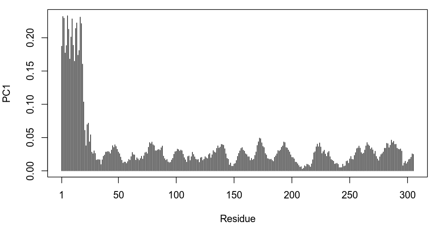
Based on the plot above we can see that the first residues in the protein are the most variable along the first component of variation. As we could have anticipated, this corresponds to the large difference in the conformation of the first helix in 6C0U_A.
Finally, we can also make an “animation” by generating several predicted structures along the axis of variation of a specific principal component. This will save the predicted structures as frames in an animation that can be visualized in Pymol.
# Make an interpolation along PC1 and save it to a file called pc1.pdb
mktrj.pca(pca_data, pc=1, file="pc1.pdb")
Exercise 9.3
Generate a similar interpolation but using instead the second principal component. Download the generated pdb file to your local computer, open it with Pymol and observe the dynamics. Try to think about what these dynamics might be for.
mktrj.pca(pca_data, pc=2, file="pc2.pdb")
In-class problems
In-class Problems Week 9
Using the information provided before, use the bio3d library to load the 7FCD structure.Before moving forward create a new structure object that only has the atoms from chain A.
Follow the same set of steps as done for the 5J5X example and perform a blast search against the PDB sequences. Retrieve the top 10 hits, align them using MUSCLE, perform a structural alignment and calculate the RMSD between them.
What is the mean RMSD among the 10 structures, approximate to the first decimal (A:5.3)
Perform the hierarchical clustering of the structural similarity using as a distance the RMSDs.
What is the structure that is most similar to 7BYR_A (A:7A25_A)
Try to understand what are the most important structural differences in the different structures of the spike protein. You can do this by opening two representative structures from the clustering analysis. A more advanced analysis would be to generate interpolated structures along the first principal complement as illustrated for the 5J5X example.