Image analysis 2
General information
Main objective
In this lesson you will learn about the foundation of image analysis. You will learn (i) basic concepts of image analysis such as image matrix, bit-depth, lookup table, histogram and threshold (ii) how to apply these concepts using ImageJ to proceed with image analysis.
Learning objectives
Learning objective 1 - You can explain the following concepts
conversions: 8- and 16-bit pseudo color images and 32-bit floating point images to RGB
multichannel images
point operations
filters
transforms
Learning objective 2 - You can perform these operations using ImageJ
converting to RGB image
use channels tool
use image calculator
use image math
use basic fileters & transfroms
Resources
Completing the image analysis part of the course requires accomplishing some exercises. All required images for these exercises should be downloaded from Github-ScopeM-teaching
Introduction to Bioimage Analysis
The content presented here is adapted from the book Introduction to Bioimage Analysis by Pete Bankhead, which can be accessed in its entirety here. We have shared this material in compliance with the Creative Commons license CC BY 4.0, the details of which can be found here. While we have only made modifications to the formatting of the excerpts, we highly recommend reading the complete book for a deeper understanding of bioimage analysis.
Color images
Types of color images
One way to introduce color into images is to use a suitable LUT, as described previously. Then the fact that different colors could be involved in the display of such images was really only incidental: at each location in the image there was still only one channel, one pixel and one value.
There are images for which color plays a more important role. We will consider two types: 1. RGB images – which are widely used for display, but are usually not very good for quantitative analysis 2. Multichannel / composite images – which are often better for analysis, but need to be converted to RGB for display
Since they often look the same, but behave very differently, knowing which kind of color image you have is important for any scientific work.
Mixing red, green & blue
We previously discussed how image LUTs provide a way to map pixel values to colors that can be displayed on screen. Now that we’ve looked at image types and bit-depths, we can expand a bit more on how that works in practice.
In general, each color is represented using three 8-bit unsigned integers: one for red, one for green, one for blue. Each integer value defines how much of each primary color should be mixed together to create the final color used to display the pixel.
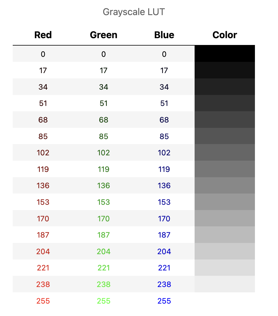
In the case of a grayscale LUT, the red, green and blue values are all the same:
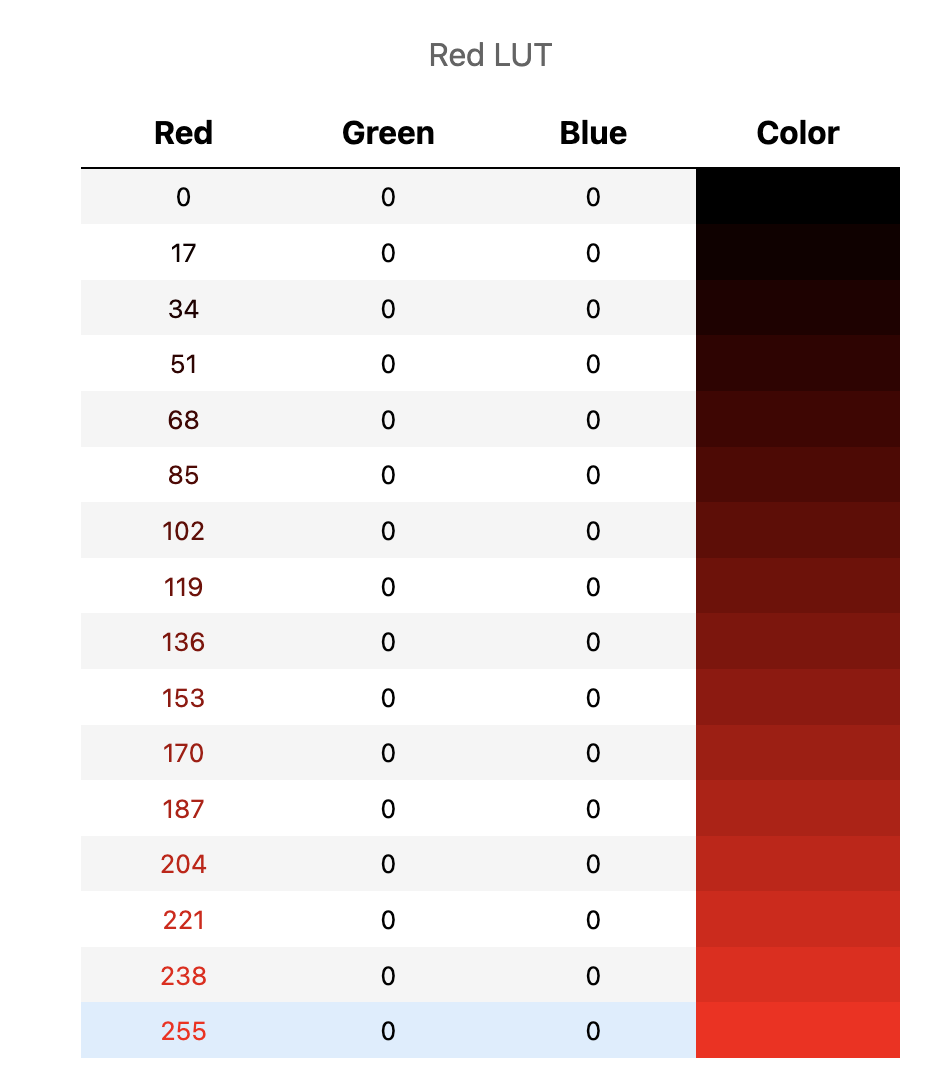
Other LUTs may include only one color, with the others set to zero:
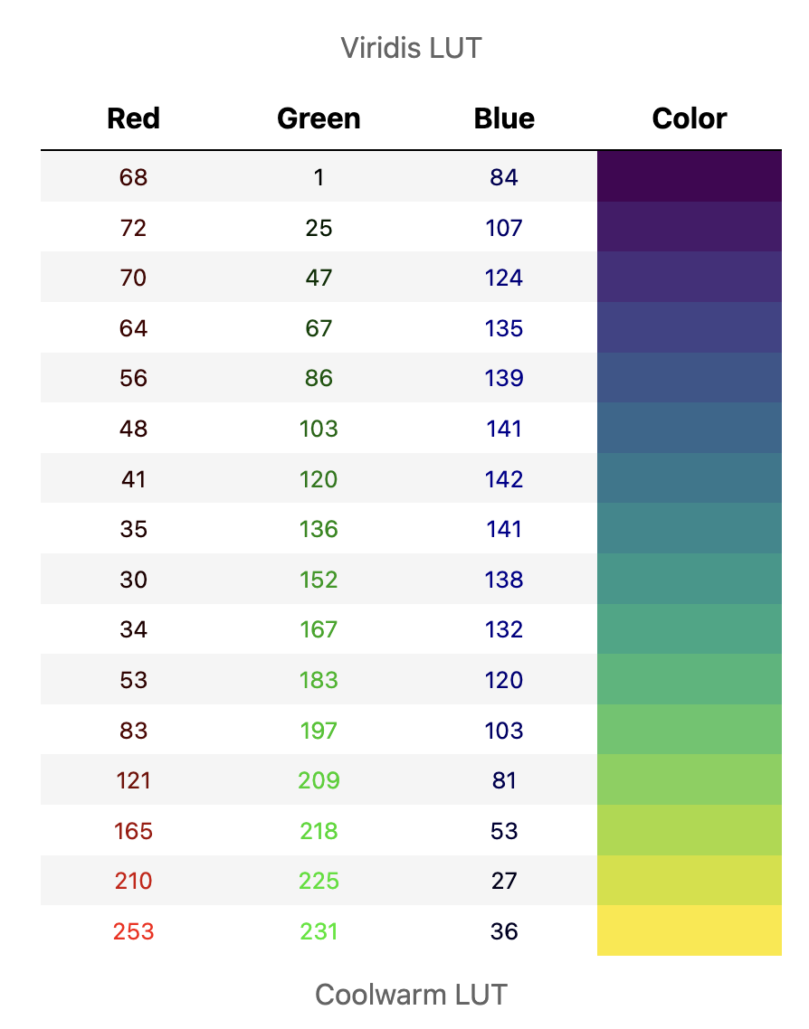
However for most LUTs the red, green and blue values differ:
Because each of the red, green and blue values can be in the range 0-255, mixing them together can generate (theoretically at least) up to 256 x 256 x 256 = 16,777,216 different colors, i.e. a lot.
When it comes to display, this method of representing color using 8-bit RGB values should easily give us many more colors than we could ever hope to distinguish by eye. We don’t need a higher bit-depth for display.
RGB images
Until now, we have considered images where each pixel has a single value, and there is a LUT associated with the image to map these values to colors.
Now that we know how colors are represented, we can consider another option.
Instead of storing a single value per pixel, we can store the RGB values that represent the color used to display the pixel instead. Each pixel then has three values (for red, green and blue), not just a single value.
When an image is stored in this way it’s called an RGB image.
We can easily create an RGB image from any combination of image + LUT: just replace each pixel value in the original image with the associated RGB values that we find in the LUT. Now each pixel has three values instead of one, but the end result looks exactly the same.
The risk of RGB
The problem with converting an image to RGB is that, in general, we can’t go back! In fact, the unwitting overuse of RGB images is one of the most common sources of data-destroying errors in some branches of scientific imaging.
Beware converting to RGB! Converting an image to RGB is another way lose our raw data.
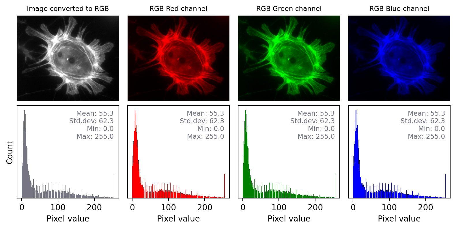
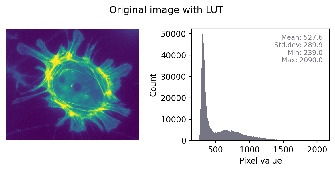
Figure below shows this in action. In the ‘least destructive’ case, the image has a grayscale LUT. This means that the red, green and blue values are identical to one another – but not necessarily identical to the pixel values of the original image. We have converted the data to 8-bit and used the LUT to determine how much to scale during the conversion.
In general, it’s not possible to recover the original pixel values from the RGB image: we probably don’t know exactly what rescaling was applied, and we have lost information to clipping and rounding.
Converting a grayscale image to RGB can lose information. We can separate out the red, green and blue values from the RGB image and visualize each as separate images to explore the information they contain. Even though the RGB image looks unchanged from the original, and all three color channels have similar histograms to the original, the bit-depth has been reduced and image statistics modified. There is also a big histogram peak that indicates substantial clipping.
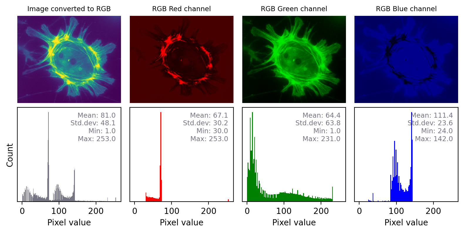
The impact of converting an image with any other LUT to RGB is even more dramatic, as shown in the previous figure. Here, the red, green and blue values are different and the histograms for each color are very different. Again, it would not be possible to recover the original pixel values from the RGB image.
Converting an to RGB can lose information in a particularly dramatic way if the LUT is not grayscale. The histograms for each channel may now look completely different.
The role of RGB
Using RGB images for display
So what’s the point of having RGB images, if they are so risky?
One of the biggest reasons to use RGB images in science is for presentation. While specialist image analysis software applications, such as ImageJ, are typically designed to handle a range of exotic image types and bit-depths, the same is not true for non-scientific software.
If you want an image to dispay exactly the same in ImageJ as in a PowerPoint® presentation or a figure in a publication, for example, we’ll probably want to convert it to RGB. If we don’t, the image might display very strangely on other software – or even not open at all.
Over the years, I have encountered a remarkable number of cases where a researcher has saved their fluorescence microscopy images only in an RGB format.
Their justification was that they tried saving the images in different way at the microscope, but ‘it didn’t work – the images were all black’.
The explanation is almost invariably that their images were really 16-bit or 32-bit, but they tried to open them in software that doesn’t handle 16-bit images very well (e.g. they just double-clicked the file to open it in the default image viewer). All they saw as a black, seemingly-empty image.
Whenever they tried exporting from the microscope’s acquisition software in different ways, they found an option that gave a viewable image – and stuck with that.
The problem with this is that it usually meant that they didn’t save their raw data at all! They only saved an RGB copy, with all the rescaling and LUT magic applied, which is wholly unsuitable for analysis.
The solution is to view images in ImageJ, or similar scientific software. This usually reveals that the image is not ‘all black’ after all. Rather, one only needs to adjust the brightness and contrast (using the LUT) to see the raw data in all its glory.
When RGB is all you’ve got
All the previous comments about ‘don’t convert to RGB before analysis’ as based on the assumption that your raw data isn’t already RGB. This is usually the case with microscopy and medical imaging whenever accurate quantification is important.
Nevertheless, it’s not always the case.
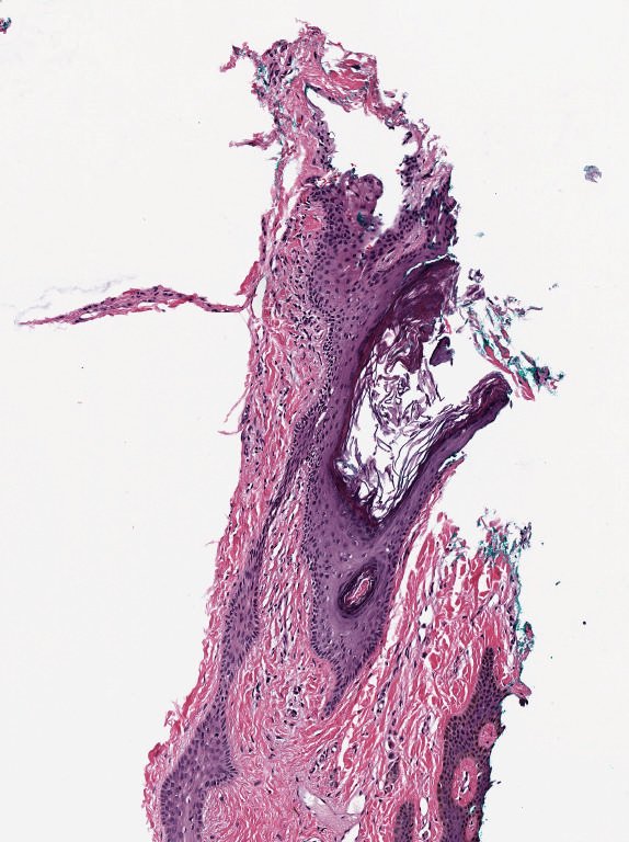
A common example is brightfield imaging for histology or pathology. Here, the camera is often RGB and an RGB image is really as close to the raw data as we are likely to get.
Example RGB histology image, from https://openslide.org
Crucially, the analysis of brightfield images in histology usually aims to replicate (and sometimes improve upon) the visual assessment that a pathologist might make looking down a microscope. It’s often based on detecting, classifying and counting cells, measuring stained areas, or recognizing the presence of particular patterns – but not accurately quantifying staining intensity.
Multichannel images
So far, we have focussed on 2D images with a single channel – that is, a single value for every pixel at every x,y coordinate in the image.
Such images can be converted to 8-bit RGB using a LUT. If we do this, then we get an image with three channels, where each channel is displayed using red, green and blue LUTs – with the colors blended together for display. But we shouldn’t do that conversion prior to analysis in case we lose our raw data.
Now, we turn to consider multichannel images that aren’t RGB images. Rather, the raw data itself has multiple channels.
In fluorescence microscopy, it’s common to acquire multichannel images in which pixel values for each channel are determined from light that has been filtered according to its wavelength. We might choose to visualize these channels as red, green and blue, but we don’t have to.
In principle, any LUT might be applied to each channel, but it makes sense to choose LUTs that somehow relate to the wavelength (i.e. color) of light detected for the corresponding channels. Channels can then be overlaid on top of one another, and their colors further merged for display (e.g. high values in both green and red channels are shown as yellow).
The important feature of these images is that the actual channel information is always retained, and so the original pixel values remain available. This means we can still extract channels or adjust their LUTs as needed.

Multichannel image from {numref}`fig-colors_composite_rgb` using different LUTs. Again, no information is lost: we can access the original pixel values, and update the LUTs if needed.

Just like with a single channel image, we can create an RGB image that allows us to visualize our multichannel image – using the LUTs to figure out which RGB values are needed to represent the color of each pixel.
Then, again if just like with the single channel image, this is problematic if we don’t keep the raw data – because we can never recover the original values from the RGB representation.

We can create an RGB image, but then we have three channels locked to red, green and blue – which have converted the original channels to 8-bit, and mixed up information due to the LUT colors used. We can no longer recover the original pixel values after converting to RGB.
Summary of color images
The main message here can be distilled into two rules:
Always use the original image for analysis
If the raw data isn’t RGB, then don’t convert it before analysis!
Create an RGB copy of your image for display
Keep the RGB copy separate, so you always retain it and the raw image
RGB images aren’t bad – we almost always need them for display, and for some imaging applications (e.g. brightfield histology) they are the best raw data we can get. But we need to be cautious if our raw data isn’t RGB, and avoid converting to RGB too early.
In the end, it’s normal to keep at least two versions of each dataset: one in the original (possibly multichannel) format, and one as RGB for display. This RGB image is normally created as the final step, after applying any processing or LUT adjustments to the original data.
Image processing & analysis
Successfully extracting useful information from microscopy images usually requires triumphing in two main battles.
The first is to overcome limitations in image quality and make the really interesting image content more clearly visible. This involves image processing, the output of which is another image. The second is to compute meaningful measurements, which could be presented in tables and summary plots. This is image analysis.
Our main goal here is analysis – but processing is almost always indispensable to get us there.
An image analysis workflow
So how do we figure out how to analyze our images?
Ultimately, we need some kind of workflow comprising multiple steps that eventually take us from image to results. Each individual step might be small and straightforward, but the combination is powerful.
I tend to view the challenge of constructing any scientific image analysis workflow as akin to solving a puzzle. In the end, we hope to extract some kind of quantitative measurements that are justified by the nature of the experiment and the facts of image formation. One of the interesting features of the puzzle is that there is no single, fixed solution.
Although this might initially seem inconvenient, it can be liberating: it suggests there is room for lateral thinking and sparks of creativity. The same images could be analyzed in quite different ways. Sometimes giving quite different results, or answering quite different scientific questions.
Admittedly, if no solution comes to mind after pondering for a while then such an optimistic outlook quickly subsides, and the ‘puzzle’ may very well turn into an unbearably infuriating ‘problem’ – but the point here is that in principle image analysis can be enjoyable. What it takes is:
a modicum of enthusiasm (please bring your own)
properly-acquired data, including all the necessary metadata (the subject of Part I)
actually having the tools at your disposal to solve the puzzle (the subject Part II)
If you’re a reluctant puzzler then it also helps to have the good luck not to be working on something horrendously difficult, but that is difficult to control.
Combining processing tools
Image processing provides a whole host of tools that can be applied to puzzle-solving. When piecing together processing steps to form a workflow, we usually have two main stages:
Preprocessing: the stuff you do to clean up the image, e.g. subtract the background, use a filter to reduce noise
Segmentation: the stuff you do to identify the things in the image you care about, e.g. apply a threshold to locate interesting features
Having successfully navigated these stages, there are usually some additional tasks remaining (e.g. making measurements of shape, intensity or dynamics). However, these depend upon the specifics of the application and are usually not the hard part. If you can identify what you want to quantify, you’re a long way towards solving the puzzle.
Fig. 56 shows an example of how these ideas can fit together.
It won’t be possible to cover all image processing tools in a book like this. Rather, we will focus on the essential ones needed to get started: thresholds, filters, morphological operations and transforms.
These are already enough to solve many image analysis puzzles, and provide the framework to which more can be added later.
Point operations
A step used to process an image in some way can be called an operation.
The simplest operations are point operations, which act on individual pixels. Point operations change each pixel in a way that depends upon its own value, but not upon where it is in the image nor upon the values of other pixels. This is in contrast to neighborhood operations, which calculate new pixel values based upon the values of pixels nearby.
While not immediately very glamorous, point operations often have indispensable roles in more interesting contexts – and so it’s essential to know how they are used, and what complications to look out for.
Isn’t modifying pixels bad?
Part I stressed repeatedly that modifying pixels is a bad thing. Since image processing is all about changing pixel values, it’s time to add a bit more nuance:
Modifying pixel values is bad – unless you have a good reason.
A ‘good reason’ is something you can justify based upon the image data. Something you could confidently include in a journal article describing how you analyzed your image, and convince a reviewer was sensible.
You should also make sure to apply the processing to a duplicate of the image, and keep the original file. That way you can always return to the original data if you need to.
Point operations for single images
Arithmetic
Pixel values are just numbers. When we have numbers, we can do arithmetic.
It should therefore come as no surprise that we can take our pixel values and change them by adding, subtracting, multiplying or dividing by some other value. These are the simplest point operations.
We encountered this idea earlier when we saw that multiplying our pixel values could [increase the brightness](sec_images_luts). I argued that this was a very bad thing because it changes our data. Our better alternative was to change the LUT instead.
Nevertheless, there are sometimes ‘good reasons’ to apply arithmetic to pixel values – better than simply brightening the appearance. Examples include:
Subtracting a constant offset added by a microscope before quantifying intensities
See {ref}`chap_macro_simulating`
Dividing by a constant so that you can convert bit-depth without clipping
See {ref}`chap_bit_depths`
However, we need to keep in mind that we’re not dealing with abtract maths but rather bits and bytes. Which makes the next question particularly important.
Exercise 12.1
Suppose you add a constant to every pixel in the image.Why might subtracting the same constant from the result not give you back the image you started with?
If you add a constant that pushes pixel values outside the range supported by the bit-depth (e.g. 0–255 for 8-bit), then the result cannot fit in the image. It’s likely to be clipped to the closest possible value instead. Subtracting the constant again does not restore the original value.
For example: 200 (original value) + 100 (constant) → 255 (closest valid value). But then 255 - 100 → 155.
Based upon this, an important tip for image processing is:
Convert integer images to floating point before
A 32-bit (or even 64-bit) floating point image is much less likely to suffer errors due to clipping and rounding. Therefore the first step of any image processing is often to convert the image to a floating point format.
Image inversion
Inverting an image effectively involves ‘flipping’ the intensities: making the higher values lower, and the lower values higher.
In the case of 8-bit images, inverted pixel values can be easily computed simply by subtracting the original values from the maximum possible – i.e. from 255.
Why is inversion useful?
Suppose you have a good strategy designed to detect bright structures, but it doesn’t work for you because your images contain dark structures. If you invert your images first, then the structures become bright – and your detection strategy might now succeed.
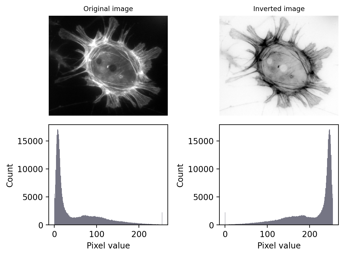
The effect of image and LUT inversion. Note that each histogram appears to be a mirror image of the other. Also, the image is clipped (sorry).
Defining the ‘maximum’ when inverting an image
Inverting an 8-bit (unsigned integer) image generally means subtracting all pixel values from 255, because 255 is the maximum supported by the image type and bit-depth.
The ‘maximum’ is not always defined in this way. For a 32-bit or 64-bit image (either integer or floating point), the maximum possible value is huge, and using that would result in exceedingly large pixel values. Therefore the ‘maximum’ is usually defined in some other way rather than based on the image type, such as by taking the maximum pixel value found within the image.
Because I don’t like letting the software decide what maximum to use, I often cheat: I multiply the pixels by -1 (ensuring the image is floating point). This retains the key properties of image inversion: it flips the high and low values, while retaining all the relative diffences between values.
Nonlinear contrast enhancement
With arithmetic operations we change the pixel values, usefully or otherwise, but (assuming we have not clipped our image in the process) we have done so in a linear way. At most it would take another multiplication and/or addition to get us back to where we were. Because a similar relationship between pixel values exists, we could also adjust the brightness and contrast LUT so that it does not look like we have done anything at all.
Nonlinear point operations differ in that they affect relative values differently depending upon what they were in the first place. These are particularly useful for contrast enhancement.
When we changed the brightness and contrast in figure, we were making linear adjustments. For a grayscale LUT, this meant we chose the pixel value to display as black and the pixel value to display as white, with each value in between mapped to a shade of gray along a straight line.
We could optionally use a nonlinear mapping values between values and shades of gray, but most software doesn’t make it straightforward to change LUTs in sufficiently complicated ways. An easier approach is to duplicate the image and apply any non-linear adjustments to the pixel values themselves, and then map them to shades of gray in the usual (linear) way.
Common nonlinear transforms are to take the logarithm of the pixel value, or replace each value \(p\) with \(p^\gamma\) where \(\gamma\) is the gamma parameter that can be adjusted depending upon the desired outcome.

Nonlinear transforms applied to a simple ‘ramp’ image, consisting of linearly increasing pixel values. Replacing each pixel with its log or gamma-adjusted value has the effect of compressing either the lower or higher intensities closer together to free up more gray levels for the others. Note that, here we assume an 8-bit input image and have incorporated some necessary rescaling for an 8-bit output (based on the approach used by ImageJ).
If all this sounds a dubious and awkward, be assured that it is: nonlinear transforms are best avoided whenever possible.
However, there is once scenario when they can really help: displaying an image with a high dynamic range, i.e. a big difference between the largest and smallest pixel values.
Figure shows this in action. Here, the pixel values associated with the main character are all quite high. However, the values associated with the ghostly figure are all very low. There are no linear contrast settings with a standard grayscale LUT that make it possible to see both figures with any detail simultaneously. However, log or gamma transforms make this possible.
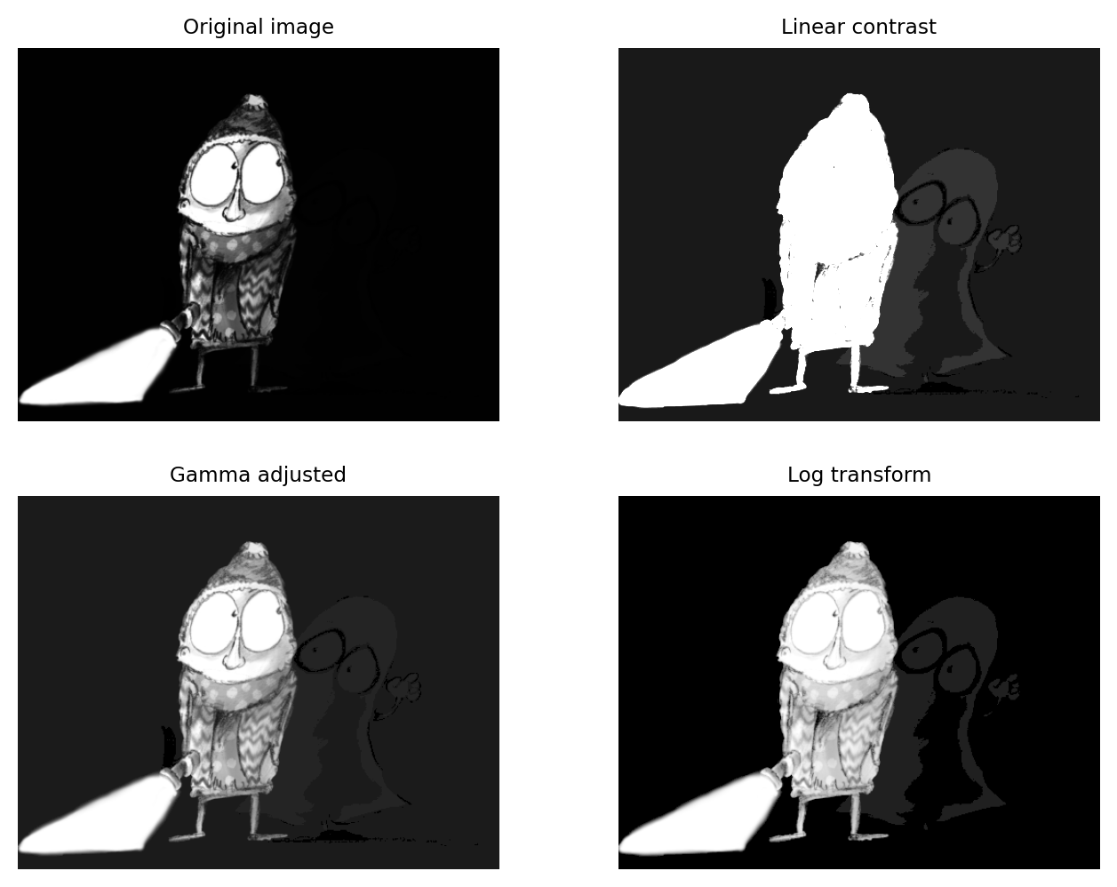
The application of nonlinear contrast enhancement to an image with a wide range of values. (Top row) In the original image, it’s not possible to see details in both the foreground and background simultaneously. (Bottom row) Two examples of nonlinear techniques that make details visible throughout the image.
Avoid image manipulation!
When creating figures for publication, changing the contrast in some linear manner is normally considered fine (assuming that it has not been done mischievously to make some inconvenient, research-undermining details impossible to discern).
But if any nonlinear operations are used, these should always be noted in the figure legend!
This is because, although nonlinear operations can be very helpful when used with care, they can also easily mislead – exaggerating or underplaying differences in brightness.
Point operations & multiple images
Instead of applying arithmetic using an image and a constant, we could also use two images of the same size. These can readily be added, subtracted, multiplied or divided by applying the operations to the corresponding pixels.
This is a technique that is used all the time in image processing. Applications include:
subtracting varying backgrounds
computing intensity ratios
masking out regions
and much more…
We will combine images in this way throughout the rest of the handbook.
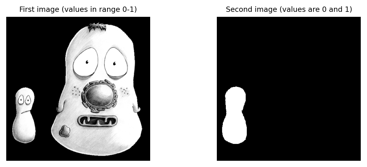
What would be the result of multiplying the images together? And what would be the result of dividing the left image by the right image?
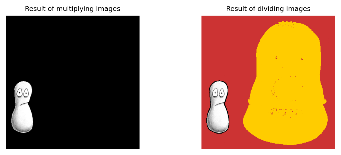
Multiplying the images effectively results in everything outside the white region in the right image being removed from the left image (i.e. set to zero).
Filters
Basics
Filters are phenomenally useful. Almost all interesting image analysis involves filtering in some way at some stage. In fact, the analysis of a difficult image can sometimes become (almost) trivial once a suitable filter has been applied to it. It’s therefore no surprise that much of the image processing literature is devoted to the topic of designing and testing filters.
The basic idea of filtering here is that each pixel in an image is assigned a new value depending upon the values of other pixels within some defined region (the pixel’s neighborhood). Different filters work by applying different calculations to the neighborhood to get their output. Although the plethora of available filters can be intimidating at first, knowing only a few of the most useful filters is already a huge advantage.
This chapter begins by introducing several extremely common linear and nonlinear filters for image processing. It ends by considering in detail some techniques based on one particularly important linear filter.
Linear filters
Linear filters replace each pixel with a linear combination (‘sum of products’) of other pixels. Therefore the only mathematical background they require is the ability to add and multiply.
A linear filter is defined using a filter kernel, which is like a tiny image in which the pixels are called filter coefficients. To filter an image, we center the kernel over each pixel of the input image. We then multiply each filter coefficient by the input image pixel that it overlaps, summing the result to give our filtered pixel value. Some examples should make this clearer.
Mean filters
Arguably the simplest linear filter is the mean filter. Each pixel value is simply replaced by the average (mean) of itself and its neighbors within a defined area.
A simple 3×3 mean filter averages each pixel with its 8 immediate neighbors (above, below, left, right and diagonals). The filter kernel contains 9 values, arranged as a 3×3 square. Each coefficient is 1/9, meaning that together all coefficients sum to 1.
The process of filtering with a 3×3 mean filter kernel is demonstrated below:

One of the main uses of a 3×3 mean filter is to reduce some common types of image noise, including Gaussian noise and Poisson noise.
We’ll discuss the subject of noise in much more detail in a later chapter, {ref}`chap_formation_noise`, and demonstrate why a mean filter works to reduce it. At this point, all we need to know about noise is that it acts like a random (positive or negative) error added to each pixel value, which obscures detail, messes with the histogram, and makes the image look grainy.
Figure illustrates of how effectively the 3×3 filter can reduce Gaussian noise in an image.

Filters can be used to reduce noise. Applying a 3×3 mean filter makes the image smoother, as is particularly evident in the fluorescence plot made through the image center. Computing the difference between images shows what the filter removed, which was mostly random noise (with a little bit of image detail as well).
Our simple 3×3 mean filter could be easily modified in at least two ways:
Its size could be increased. For example, instead of using just the pixels immediately adjacent to the one we are interested in, a 5×5 mean filter replaces each pixel by the average of a square containing 25 pixels, still centered on the main pixel of interest.
The average of the pixels in some other shape of region could be computed, not just an _n×n_ square.
Both of these adjustments can be achieved by changing the size of the filter kernel and its coefficients.
One common change is to make a ‘circular’ mean filter. We can do this by defining the kernel in such a way that coefficients we want to ignore are set to 0, and the non-zero pixels approximate a circle. The size of the filter is then defined in terms of a radius value ({numref}`fig-filter_shapes`).

The kernels used with several mean filters. Note that there’s no clearly ‘right’ way to approximate a circle within a pixel grid, and as a result
different software can create circular filters that are slightly different. Here, (B) and (C) match the ‘circular’ filters used by ImageJ’s {menuselection}Process --> Filters --> Mean... command.
Filtering at image boundaries
If a filter consists of more than one coefficient, the neighborhood will extend beyond the image boundaries when filtering some pixels nearby. We need to handle this somehow. There are several common approaches.
The boundary pixels could simply be ignored and left with their original values, but for large neighborhoods this would result in much of the image being unfiltered. Alternative options include treating every pixel beyond the boundary as zero, replicating the closest valid pixel, treating the image as if it is part of a periodic tiling, or mirroring the internal values ({numref}fig-filter_boundaries).

Different software can handle boundaries in different ways. Often, if you are using an image processing library to code your own filtering operation you will be able to specify the boundary operation.
Nonlinear filters
Linear filters involve taking neighborhoods of pixels, scaling them by the filter coefficients, and adding the results to get new pixel values. Nonlinear filters also make use of neighborhoods of pixels, but can use any other type of calculation to obtain the output. Here we’ll consider one especially important family of nonlinear filters.
Rank filters
Rank filters effectively sort the values of all the neighboring pixels in ascending order, and then choose the output based upon this ordered list.
Perhaps the most common example is the median filter, in which the pixel value at the center of the list is used for the filtered output.

Results of different 3×3 rank filters when processing a single neighborhood in an image. The output of a 3×3 mean filter in this case would also be 15.
Image transforms
An image transform converts an image into some other form, in which the pixel values can have a (sometimes very) different interpretation.
There are lots of ways to transform an image. We will focus on two that are especially useful for bioimage segmentation and analysis: the distance transform and the watershed transform. We will briefly introduce both, before then showing how they can be used in combination.
The distance transform
The distance transform (sometimes called the Euclidean distance transform) replaces each pixel of a binary image with the distance to the closest background pixel.If the pixel itself is already part of the background then this is zero. The result is an image called a distance map.
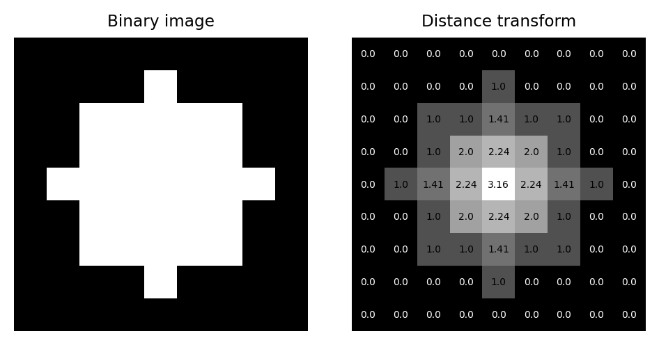
A binary image and its corresponding distance map, including pixel values as an overlay.
A natural question when considering the distance transform is: why?
Although its importance may not be initially obvious, we will see that creative uses of the distance transform can help solve some other problems rather elegantly.
For example, eroding or dilating binary images by a large amount can be very slow, because we have to use large maximum or minimum filters. However, erosion and dilation can be computed from a distance map very efficiently simply by applying a global threshold. This can be much faster in practice.
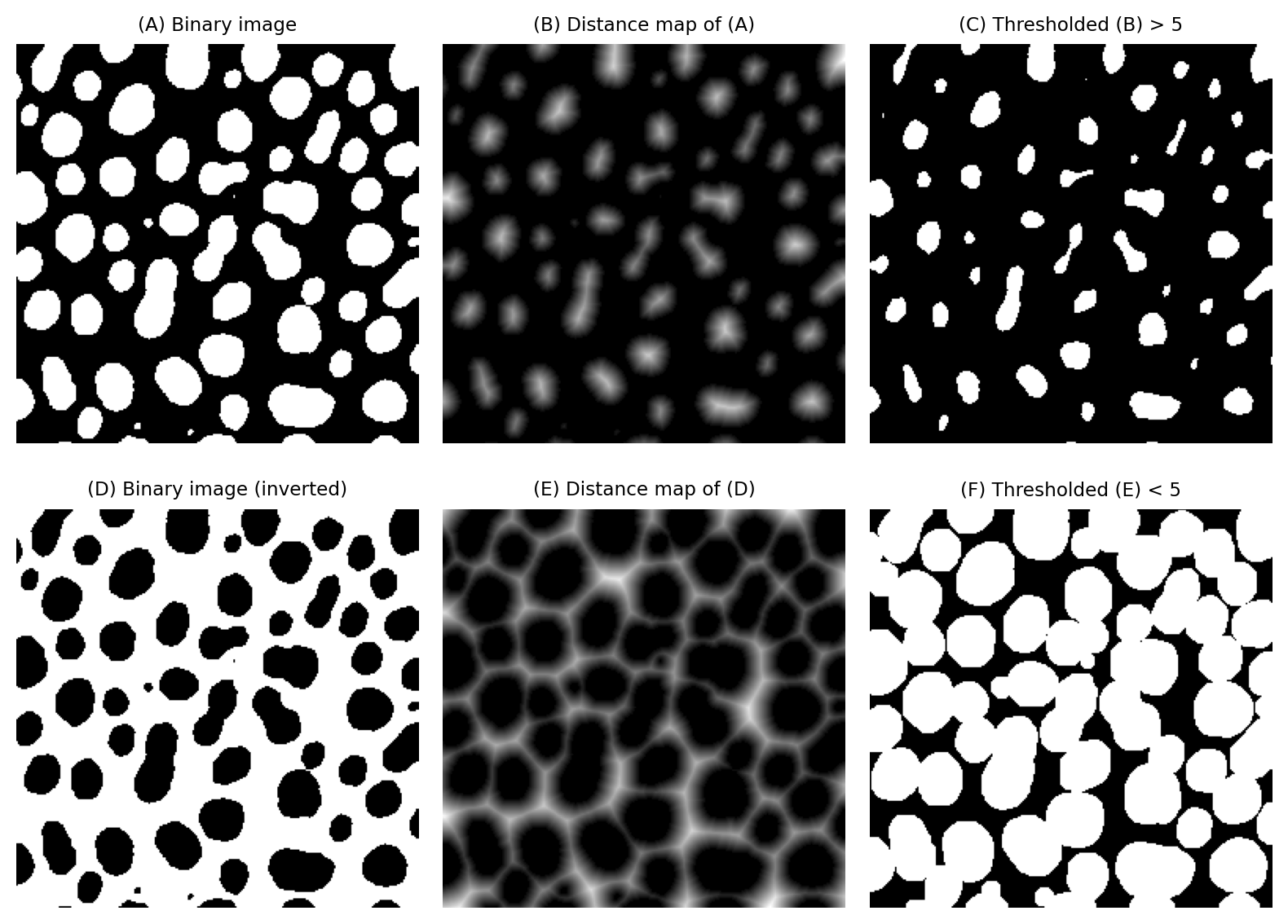
Implementing erosion (C) and dilation (F) of binary images by thresholding distance maps.
But the distance map contains useful information that we can use in other ways.
For example, we can also use distance maps to estimate the local thickness of a structure. An application of this would be to assess blood vessel diameters. If we have a binary image representing a vessel, we can generate both a distance map and a thinned binary image. The distance map values corresponding to foreground pixels in the thinned image provide a local estimate of the vessel radius at that pixel, because the distance map gives the distance to the nearest background pixel – and thinned pixels occur at the vessel center.
However, the distance transform can become even more useful if we combine it with other transforms.
The watershed transform
The watershed transform is an example of a region growing method: beginning from some seed regions, the seeds are progressively expanded into larger regions until all the pixels of the image have been processed. This provides an alternative to straightforward thresholding, which can be extremely useful when need to partition an image into many different objects.
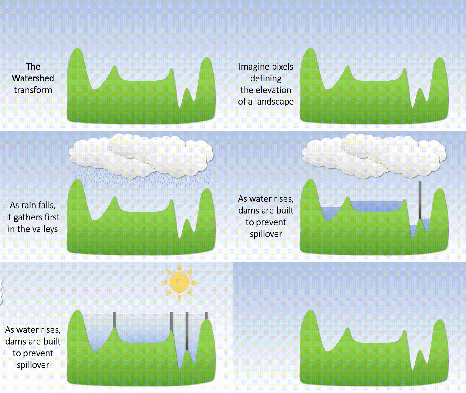
To understand how the watershed transform works, picture the image as an uneven landscape in which the value of each pixel corresponds to a height.

Visualizing an image as a landscape, using surface plots. Higher pixel values are generally viewed as peaks, although can easily switched to become valleys by inverting the image before plotting. This may be useful when providing input to the watershed transform.
Now imagine water falling evenly upon this surface and slowly flooding it. The water gathers first in the deepest parts; that is, in the places where pixels have values lower than all their neighbors. These define the seeds of the watershed transform; we can think of them as separate water basins.
As the water level rises across the image, occasionally it will reach a ridge between two basins – and, in reality, water could spill from one basin into the other. However, in the watershed transform this is not permitted; rather a dam is constructed at such ridges. The water then continues to rise, with dams being built as needed, until in the end every pixel is either part of a basin or a ridge, and there are exactly the same number of basins afterwards as there were at first.
Applying the watershed transform to an image. Here, we passed the inverted image to the watershed transform because we want to identify bright spots rather than dark ones. The full watershed transform will expand the seeds to create a labeled image including all pixels, but we can optionally mask the expansion to prevent it filling the background. Here, we defined the mask by applying a global threshold using the triangle method. Note that the masked watershed segmentation is able to split some spots that were merged using the global threshold alone.
Crucially, as the seeds are expanded during the watershed transform, regions are not allowed to overlap. Furthermore, once a pixel has been assigned to a region then it cannot be moved to become part of any other region.
Using the ‘rain falling on a surface’ analogy, the seeds would be regional minima in an image, i.e. pixels with values that are lower than all neighboring pixels. This is where the water would gather first.
In practice, we often need to have more control over the seeds rather than accepting all regional minima (to see why too many local minima could be a problem, observe that {numref}`fig-transform_surface_watershed` contains more regions that we probably would want). This variation is called the seeded watershed transform: the idea is the same, but we simply provide the seeds explicitly in the form of a labeled image, and the regions grow from these. We can generate seeds using other processing steps, such as by identifying [H-minima](sec_h_extrema).
Combining transforms
The watershed transform can be applied to any image, but it has some particularly interesting applications when it is applied to an image that is a distance map.
Splitting round objects
A distance map has regional maxima whenever a foreground pixel is further from the background than any of its neighbors.
This tends to occur towards the center of objects: particularly round objects that don’t contain any holes. Importantly, regional maxima can still be present even if the ‘round objects’ are connected to one another in the binary image used to generate the distance map originally.
This means that by applying a watershed transform to a distance map, we are able to split ‘roundish’ structures in binary images. The process is as follows:
Compute the distance map of the image
Invert the distance map (e.g. multiply by -1), so that peaks become valleys
Apply the watershed transform, starting from the regional minima of the inverted distance map

Splitting round objects using the distance and watershed transforms.
In-class problems
In-class Problems Week 12
For the homework, you are required to take the quiz Image analysis 2 - Quiz that is posted on Moodle under ‘Quizzes’.
