Image analysis 1
General information
Main objective
In this lesson you will learn about the foundation of image analysis. You will learn (i) basic concepts of image analysis such as image matrix, bit-depth, lookup table, histogram and threshold (ii) how to apply these concepts using ImageJ to proceed with image analysis.
Learning objectives
Learning objective 1 - You can explain the following concepts
ImageJ & Fiji
image matrix
simplified image formation for fluorescent images
lookup table
image histogram
image normalization
conversions: 8- and 16-bit pseudo color images and 32-bit floating point images
threshold
Learning objective 2 - You can perform these operations using ImageJ
installing Fiji, updating it and adding plugins
peeking into image matrix using pixel inspection tool
changing lookup tables
displaying image histogram
changing the look of the image by using Image / Adjust / Brightness and Contrast tool
converting the image to 8/16/32-bits
applying Threshold
using Analyze Particles tool to count objects
Resources
Completing of the image analysis part of the course requires accomplishing some exercises. All required images for these exercises should be downloaded from Github-ScopeM-teaching
Introduction to Bioimage Analysis
The content presented here is adapted from the book Introduction to Bioimage Analysis by Pete Bankhead, which can be accessed in its entirety here. We have shared this material in compliance with the Creative Commons license CC BY 4.0, the details of which can be found here. While we have only made modifications to the formatting of the excerpts, we highly recommend reading the complete book for a deeper understanding of bioimage analysis.
ImageJ
What is ImageJ?
ImageJ is open-source software for image analysis.
Created by Wayne Rasband at the National Institutes of Health, ImageJ has become indispensable to the research community over more than 20 years. It continues to be updated regularly and is by far the most discussed topic on the Scientific Community Image Forum – with more than 10,000 topics at the time of writing, and more added every day.
ImageJ’s success is due not only to the features of the software itself, but to its openness and extensibility. The source code is in the public domain, meaning that others can adapt it as needed. But usually this isn’t necessary, because users can write (and share) custom macros, plugins or scripts to add new functionality – without changing ImageJ itself.
Getting ImageJ
ImageJ is available in multiple forms. Three of the most important ones for our purposes are:
1. ImageJ
Download from https://imagej.nih.gov/ij/
The ‘original’ download of ImageJ contains all the core functionality, but no extra user plugins.
The core of the application is a tiny file ij.jar (~2.5 MB) that runs on Java. You can download a platform-specific package that includes both ImageJ and Java for Windows, Mac or Linux. Including Java makes the download bigger, but makes the application self-contained and easy to run.
2. Fiji

Download from https://fiji.sc/
Fiji, which stands for Fiji Is Just ImageJ, is a distribution of ImageJ that comes bundled with a plethora of plugins and extra features that are especially useful for life scientists. It also has a powerful script editor that helps a lot when developing macros or scripts, an updater to help manage all the additions, and even a ‘Big Data Viewer’ for particularly huge images.
3. ImageJ.JS
Run at https://ij.imjoy.io
ImageJ.JS is a web version of the original ImageJ, capable of running in a browser. It has a few extra features, but not as many as Fiji. It was put together and is maintained by the ImJoy team led by Wei Ouyang.
For more information, see https://imagej.net/software/imagej-js
More interactivity with ImageJ.JS!
Whenever you see a button like this it can be used to launch ImageJ.JS directly from this page, often with a relevant image opened.
By default, ImageJ.JS will open in the same browser tab. If you want it to open in a new tab, then there’s probably an easy trick in your browser to do that (on a computer, my guess is that it’ll be pressing Ctrl or ⌘ when clicking the link).
Remember to cite the software you use!
A lot of open-source software is developed and supported by academics, who invest a huge amount of time into development and support. They need funding to continue that work, and paper citations to help get that funding.
If you use software for research you plan to publish, please spend a few minutes searching for how the developers of the software want it to be cited.
For ImageJ & Fiji, see https://imagej.net/contribute/citing
For other software, google for citing [software name]
Sometimes they also need a kind word or a compliment, because they are human. Supporting software can be time-consuming, hard and stressful – and is usually something they do for free, in their limited spare time.
The ImageJ Interface
ImageJ’s user interface is rather minimalistic.
It’s centered around a toolbar.
Everything else (images, histograms, measurement tables, dialogs) appears within separate windows. Please open Fiji or and experiment while reading the description below.
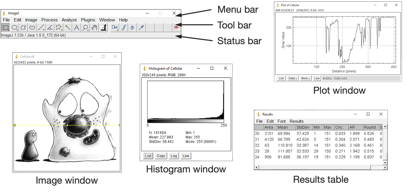
But despite the simple appearance, ImageJ is powerful. The depth of the software is evident from its abundance of menus and submenus.
That leads to the most important tip for using ImageJ:
Search
Don’t memorize the menus – search!
ImageJ has a lot of options, buried in a lot of menus… and submenus… and sometimes sub-submenus.
Fortunately, there’s no reason to memorize where they all are to be found. Rather, just remember one shortcut key: L
Pressing L effectively brings up a list of all the commands from the menus, ready for each search.
For ImageJ, you see the Command Finder window where you can begin to type the name of the command you want. You can then run it either by double-clicking on the entry, or by using the up or down arrow keys followed by Enter.
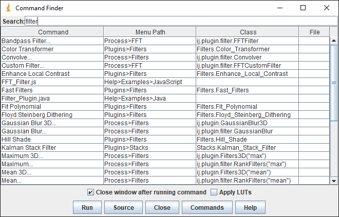
In Fiji, you might see the Command Finder or you can alternatively switch on a search bar by selecting it under Edit –> Options –> Search Bar... The idea is the same. The search bar can also be activated using L and used to find and run commands.
Shortcuts
In most software, shortcut keys often require pressing Ctrl (on Windows, Linux) or ⌘ (Mac). Therefore the shortcut to search for a command would be Ctrl + L or ⌘ + L.
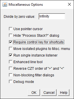
This works in ImageJ, but isn’t necessary. Under Edit –> Options –> Misc.., you can specify whether the Ctrl or ⌘ key is needed along with the letter for the shortcut.
By default, this option is turned off – so pressing L alone is enough. You may find this might make it too easy to accidentally run commands, in which case you should select the option to turn it on.
Opening images & viewing pixels
I am always taken aback when I see someone open an image in ImageJ through the menus, by choosing File –> Open...
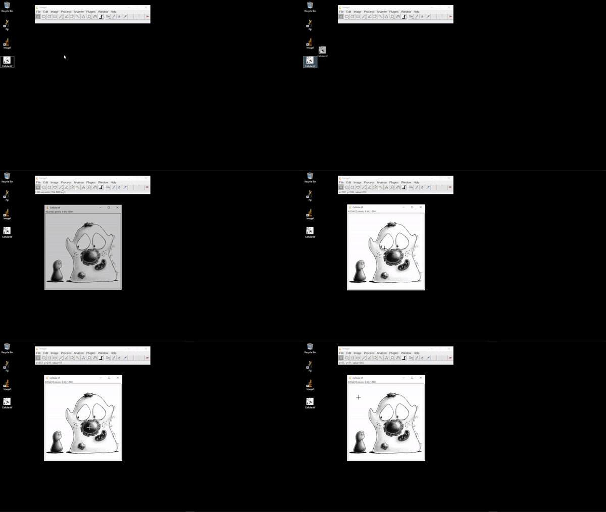
Although this can work, it’s unnecessarily slow and awkward. The more elegant way to open an image is to simply drag the image file onto ImageJ’s toolbar.
As the cursor is then moved over the image, the value for the pixel under the cursor is displayed in ImageJ’s status bar. Images can be navigated as follows:
Zoom in
Select the
 tool, then left-click on the image, or
Press the + key
Zoom out
Select the
 tool, then right-click on the image, or
Press the - key
Pan
Select the
 tool, then click and drag on the image, or
Press the spacebar, then click and drag on the image
When the image is larger than the visible region, a small (purple) overview appears in the top left to indicate which part can currently be seen.
Exercise 11.1
The status bar also shows the x and y coordinates for the pixel under the cursor. However, to interpret these you need to know the origin, i.e. the location of the pixel at x=0, y=0.
Where is the origin of the image in ImageJ?
Top left corner
Top right corner
Bottom left corner
Bottom right corner
Image center
Tip: You should be able to answer this question by opening an image in ImageJ, and observing the coordinates in the toolbar as you move the cursor over the image.
Images & pixels
Images are composed of pixels.
The word ‘pixel’ is derived from a picture element and, as far as the computer is concerned, each pixel is just a number.
When the image data is displayed, the values of pixels are usually converted into squares of particular colors – but this is only for our benefit.
The colored squares are nothing more than a helpful visualization that enables us to gain a fast impression of the image contents, i.e. the approximate values of pixels and where they are in relation to one another.
When it comes to processing and analysis, we need to get past the display and delve into the real data: the numbers.
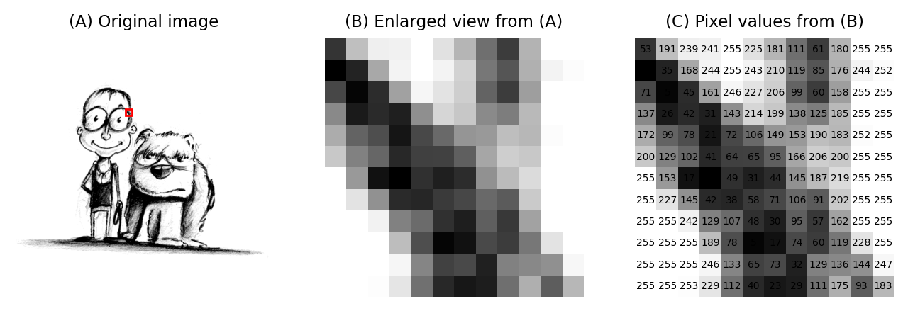
(A) & (B) The image is shown using small squares of different shades of gray, where each square corresponds to a single pixel. This is only a convention used for display; the pixels themselves are stored as arrays of numbers (C) – but looking at the numbers directly it’s pretty hard for us to visualize what the image contains.
Image data & its display
The distinction between a pixel’s numeric value and the color used to display it might seem like a minor detail, but it definitely isn’t: failing to recognize this difference underlies a lot of errors.
If we aren’t careful, two related facts can cause us an enormous amount of trouble:
Warning:
Images that look the same can contain different pixel values
Images that look different can still contain the same pixel values

Images that look the same, but contain different pixel values. Measuring each of these images would give different results, for reasons we shall see in later chapters.

Images that look different, but contain the same pixel values. Measuring each of these images would give the same results.
This is crucial because it’s entirely possible to analyze two different images that appear identical, but to get very different (and very wrong) results.
This is far from a theoretical problem. It happens a lot in practice whenever someone innocently makes an adjustment to an image (e.g. to make it look brighter, or change the colors for display) without realizing that the adjustment has actually changed the pixel values – and thereby compromised the underlying data. This can fatally undermine the integrity of any later analysis.
What’s worse, these errors can go completely unnoticed, surreptitiously compounding the problem of reproducibility in science.
This brings us to the key message of this chapter:
Don’t (just) trust your eyes!: In science, we need to know what is happening whenever we open, adjust and save our images. If we don’t, we risk misinterpreting our data.
Fortunately, knowing just a little bit about imaging and image analysis is enough to avoid making these mistakes. Knowing more than a little bit can open up new worlds of possibility to extract useful information from scientific images.
We’ll start by considering two questions:
Where do the pixel values come from?
How are pixel values converted into colors for display?
It’s hard to give a detailed-but-general answer to the first question, because the origin and interpretation of the pixel values depend upon how the image was created, and there are many different ways to generate an image.
Nevertheless, the key ideas are similar everywhere. By way of illustration, we’ll consider a very common case in bioimaging where the pixel values relate to detected light – specifically, using the example of a fluorescence microscope – before moving how to see how these values are displayed.
A simple microscope
When I work with fluorescence images, I have a very simple picture in my head of how the image is formed. It may not be very exact, but I find it extremely useful as a basis to which we can add detail whenever we need it. We will revisit this picture later in the book to help organize the interrelating imaging considerations relevant to the analysis.
In my simplified model, there are only three components that we need to worry about:
Sample – the thing we want to look at
Objective lens – the thing that gathers the light and focuses it for detection
Detector – the thing that detects the light to form the digital image (here, a CCD camera)
The process is illustrated below:
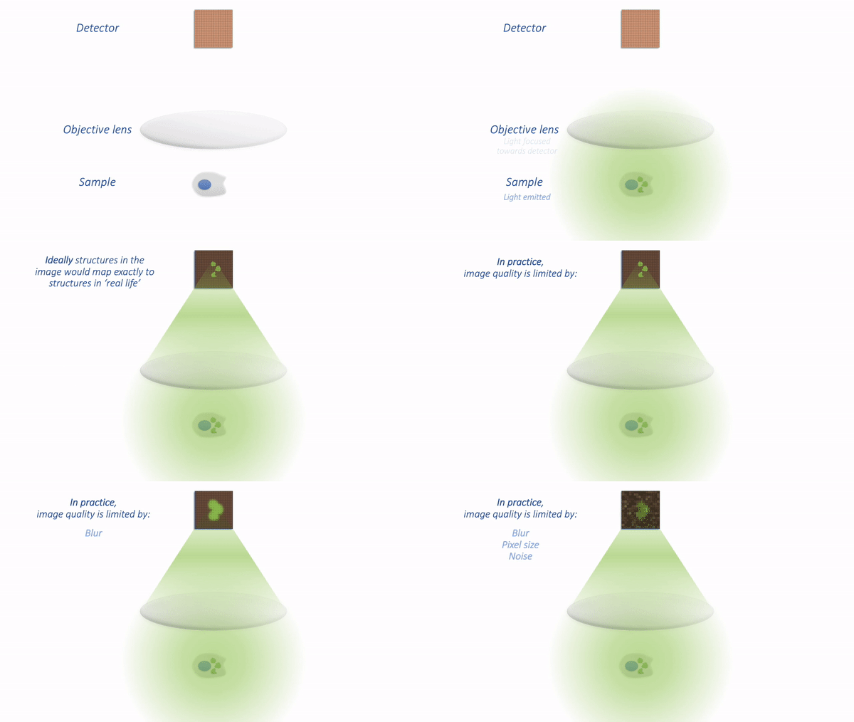
Simple microscope.
There are a couple of things to note at this point:
Not all the light emitted from the sample is detected. A lot of it never enters the objective lens.
Our images aren’t perfect. We will explore problems of blur, noise and pixel size later.
For now, we are mostly interested in the detection step and how it generates a digital image. Zooming in to look at this in more detail, we can imagine what happens as light hits the camera. The sensor of the camera itself is divided into physical pixels, which will correspond to the pixels in the final image. When a photon strikes the detector, an electron may be released at one of the physical pixels. During the acquisition of an image, many photons strike the detector, which can cause many electrons to be released at different physical pixels. These electrons contribute to the value of a pixel in the final image: more electrons → higher pixel values.
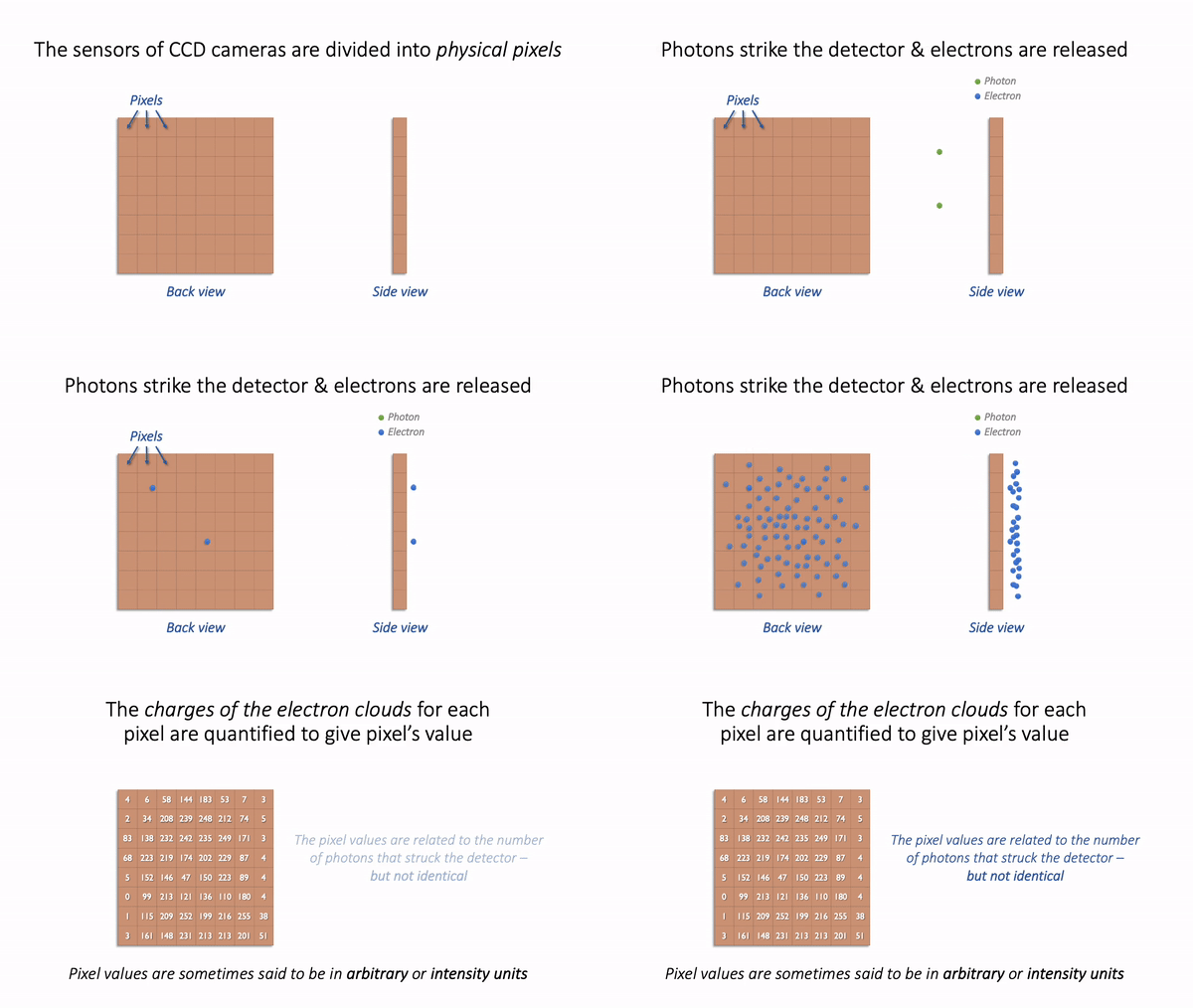
Simple camera.
The important point is that pixel values are only *indirectly* related to whatever it is in our sample that we want to measure.
In this example, they have been derived by quantifying the charge of electron clouds gathered at each physical pixel. This should be proportional to the amount of detected light that originated from a particular volume of the sample. This, in turn, depends upon what is actually present in the sample – but there are a lot of things that can influence the final values in connection with acquisition parameters, conversion factors, and physics. These are not usually related directly to the thing you might want to quantify.
Some of the factors influencing pixel values:
Amount of time spent detecting photons
More time –> More photons –> More electrons –> Higher pixel values
Numerical aperture of the objective lens
This relates to the angle of light accepted by the objective
Higher NA –> Larger angle –> More photons –> More electrons –> Higher pixel values
Sensitivity of the detector (Quantum Efficiency)
Not all photons necessarily produce an electron; I think of this as the photon hitting the detector, but not hard enough to dislodge an electron. A detector with low sensitivity is likely to ‘miss’ more photons, so that they never contribute to the pixel value.
Higher sensitivity –> More electrons –> Higher pixel values
Ultimately, this leads to the warning: Don’t over-interpret pixel values! Individual pixel values are rarely very meaningful in isolation: we’re usually interested in relative differences between groups of pixels.
As we shall see, this means that we often need to average values and normalize to something whenever we want to make measurements in an image. We can’t usually untangle the influences well enough to infer anything with confidence from a single pixel value.
But the limitations in what pixel values can tell us don’t diminish their importance: on the contrary, pixel values remain our raw data and it’s essential that we preserve them as faithfully as possible. That’s a lot harder than you might expect. It requires knowing when and how pixel values might become changed whenever we are working with our images. This is so crucial that it will be the focus throughout the entire first part of this book.
Lookup tables
Lookup tables are sometimes referred to as colormaps.
For our purposes, the terms are interchangeable – you may see either depending upon which software you are using.
So images are really comprised of a lot of numbers – the pixel values – even though we normally visualize them as shapes and colors.
It’s time then to consider our second question: How are pixel values converted for display?
The basic idea is simple: the software displaying the image uses a lookup table (LUT) that maps each pixel value to a color. When it comes to showing the image, each pixel is replaced by a little dot or square on the screen that has the corresponding color.
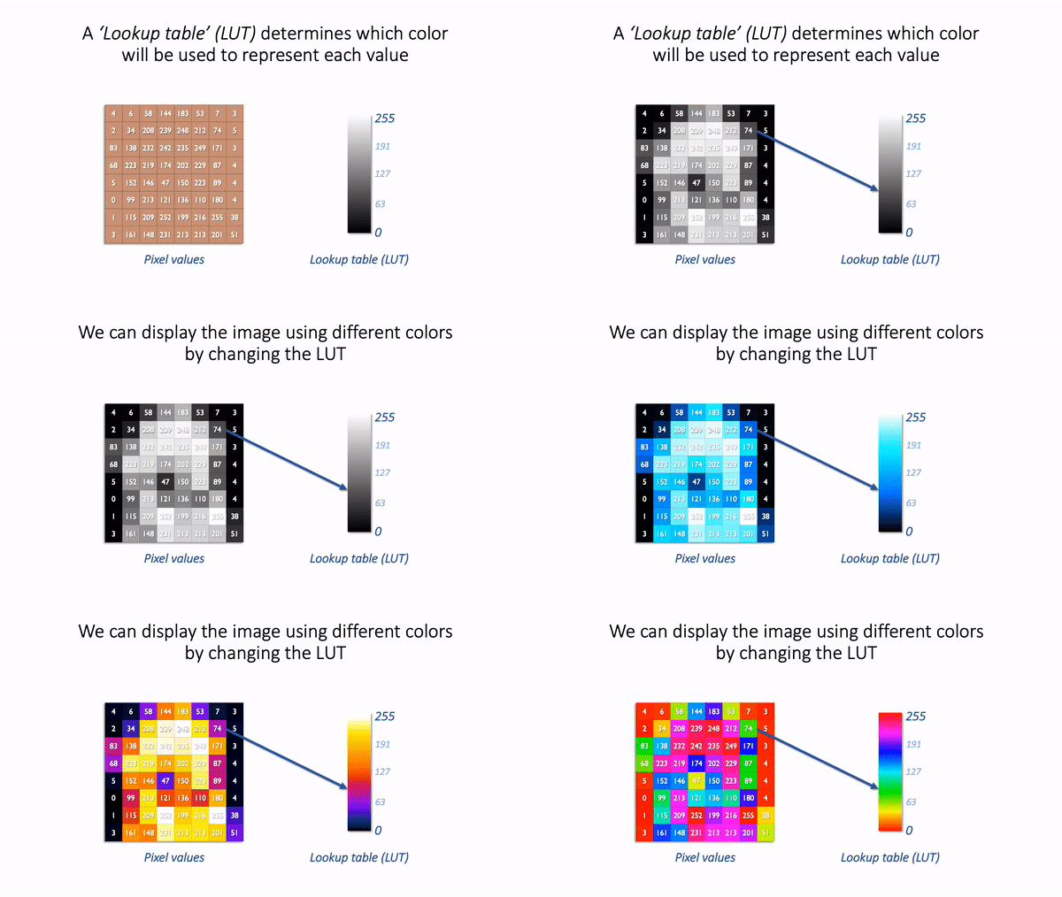
LUT concept.
LUTs therefore provide a way to change the appearance of an image without changing its pixel values.
This is extremely useful in practice. Since images in biology often have rather low pixel values (formed from a small amount of detected light), we very often want to change their brightness for the display.
One way we could make an image brighter is to change the pixel values themselves – multiply them by 2, for example. That would indeed usually make the image look brighter, but we risk making a terrible mess of our data if we permit ourselves to make such changes. As described above, we really don’t want to modify our raw data unnecessarily.
A much better way to change the brightness of an image is to change the LUT only.
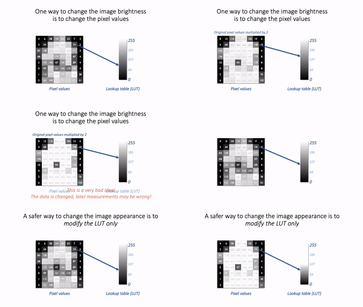
The danger is that not all software cares so much about preserving pixel values. Someone wanting to enhance their holiday photos isn’t likely to care about retaining the original pixel values for quantification later; rather, they just want the images to look as nice as possible.
For this reason, a lot of software designed for working with images really will rescale the pixel values when you do something as simple as adjusting the brightness. And so it is entirely possible to open an image, adjust the display slightly to see things more clearly, and in doing so irreparably damage the image – losing the raw data required for later analysis.
This is why you should use scientific software for scientific image analysis – and not just any general imaging editing software you might find.
But even when using scientific software, it’s often possible to change pixel values whenever you’d really rather only be changing lookup tables. The next chapter will show how to check when this is happening.
Changing image appearance
Switching LUTs
You can change the colors of the LUT by selecting an alternative option from the Image –> Lookup tables submenu.
Use the Control Panel to frequently access the same menu: If you want to explore LUTs quickly, use Plugins –> Utilities –> Control Panel. This opens a window that allows you to double-click on commands from any menu or submenu to apply that command quickly.
Adjusting Brightness & Contrast
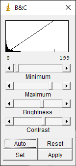
The main command to change the brightness of an image is Image –> Adjust –> Brightness/Contrast... Since you’re likely to use it a lot, it is worth learning the shortcut: Shift + C.
The Brightness/Contrast dialog has four sliders: Minimum, Maximum, Brightness & Contrast. They are linked together: changing either of the first two also results in a change to the last two, and vice versa.
Supposing you have a grayscale LUT, with colors ranging from black to white, you should see that
All pixels with a value less than or equal to the Minimum will be shown as black
All pixels with a value greater than or equal to the Maximum will be shown as white
All other pixels with a value in between will be shown using a shade of gray
Use the minimum & maximum sliders: Despite the name of the command implying Brightness and Contrast are the star performers, I would argue that the Minimum and Maximum sliders are far more intuitive.
I use Minimum and Maximum almost exclusively.
Histograms
Before we have demonstrated how looks can be deceiving: the visual appearance of an image isn’t enough to determine what data it contains.
Because scientific image analysis depends upon having the right pixel values in the first place, this leads to the important admonition: Keep your original pixel values safe! The pixel values in your original image are your raw data: it’s essential to protect these from unwanted changes.
This is really important because there are lots of ways to accidentally compromise the raw data of an image – such as by using the wrong software to adjust the brightness and contrast, or saving the files in the wrong format. This can cause the results of an analysis to be wrong.
What makes this especially tricky is that trustworthy and untrustworthy images can look identical. Therefore, we need a way to see beyond LUTs to compare the content of images easily and efficiently.
Comparing histograms & statistics
In principle, if we want to compare two images we could check that every corresponding pixel value is identical in both images. We will use this approach later, but isn’t always necessary.
There are two other things we can do, which are often much faster and easier:
Calculate some summary statistics from the pixel values, such as the average (mean) pixel value, standard deviation, minimum and maximum values.
Check out the image histogram. This graphically depicts the distribution of pixel values in the image.
Putting these into action, we can recreate previous figure but this time we add:
the LUT (shown as a colored bar below the image)
a histogram
summary statistics
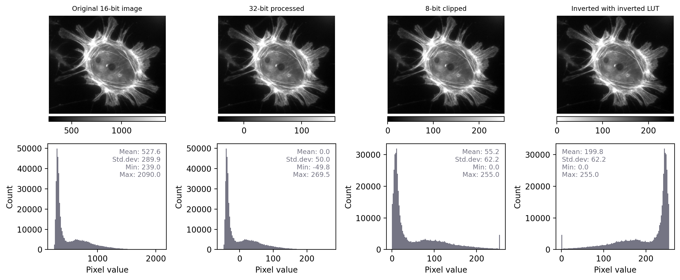
With the additional information at our disposal, we can immediately see that the images really do contain different underlying values – and therefore potentially quite different information – despite their initial similar appearance. We can also see that the LUTs are different; they show the same colors (shades of gray), but in each case these map to different values.
By contrast, when we apply the same steps we see that the histograms and statistics are identical – only the LUT has been changed in each case. This suggests that any analysis we perform on each of these images should give the same results, since the pixel values remain intact.
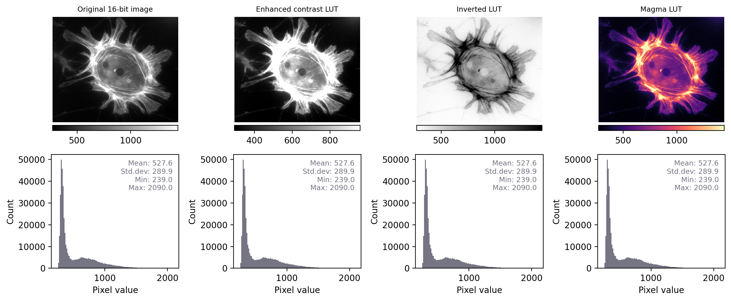
Images that look different, but contain the same pixel values – this time with measurements and histograms included.
Exercise 11.3
Question: If two images have identical histograms and summary statistics (mean, min, max, standard deviation), does this prove that the images are identical?
No! For example, we might have the same pixel values in a different arrangement. If I randomly shuffle the pixels in the image then the basic statistics and histogram remain unchanged – but the image itself is very different.
This means that, technically, we can only really use histograms and summary measurements to prove that images are definitely not the same.
However, in practice this is usually enough. If two images have identical histograms and summary statistics and look similar, it is very likely that they are the same.
Conceivably, someone might try to deceive us by making some very subtle change to an image that preserves the statistics, such as swapping two pixels amongst millions so that we don’t notice the difference.
Later, we’ll see how to overcome even that by checking every single pixel – but such elaborate trickery probably isn’t a very real risk for most of us.
Most of the time, when things go wrong with scientific images the histogram and statistics will be compromised in an obvious way – we just need to remember to check for these changes.
Types & bit-depths
As described previously, each pixel has a numerical value – but a pixel cannot typically have just any numerical value it likes. Instead, it works under the constraints of the image type and bit-depth.
Ultimately the pixels are stored in some binary format: a sequence of bits (binary digits), i.e. ones and zeros. The bit-depth determines how many of these ones and zeros are available to store each pixel. The type determines how these bits are interpreted.
Representing numbers with bits
Suppose Bob is developing a secret code to store numbers, but in which he is only allowed to write ones and zeros. If he is only allowed a single one or zero (i.e. a single bit), he doesn’t have many options.
Dec. |
Bin. |
|---|---|
0 |
0 |
1 |
1 |
Assuming he wants his encoded numbers to be consecutive integers starting from zero, this means he can only represent two different numbers: one and zero.
If he is allowed an extra bit, suddenly he can represent 4 numbers by combining the ones and zeros differently.
Dec. |
Bin. |
|---|---|
0 |
00 |
1 |
01 |
2 |
10 |
3 |
11 |
Clearly, the more bits Bob is allowed, the more unique combinations he can have – and therefore the more different numbers he can represent in his code.
With 8 bits are his disposal, Bob can combine the bits in 256 different ways to represent 256 different numbers.
Dec. |
Bin. |
|---|---|
0 |
00000000 |
1 |
00000001 |
2 |
00000010 |
3 |
00000011 |
4 |
00000100 |
5 |
00000101 |
The pixel values in an image are stored using a code just like this. Each possible value is represented in binary as a unique combination of bits.
Image bit-depth
The bit-depth of an image is the number of bits used to represent each pixel. A bit-depth of 8 would indicate that 8 bits are used to represent a single pixel value.
The bit-depth imposes a limit upon the pixel values that are possible. A lower bit-depth implies that fewer different pixel values are available, which can result in an image that contains less information.

Representing an image using different bit-depths.
As shown previously, a 1-bit image can contain only two values: here, shown as black or white pixels. Such binary images are extremely limited in the information that they can contain, although will turn out to be very useful later when processing images.
A 2-bit image is not much better, containing at most only 4 different values. A 4-bit image can have 16 values. When visualized with a grayscale LUT, this is a substantial improvement. In fact, the eye is not particularly good at distinguishing different shades of gray – making it difficult to see much difference between a 4-bit and 8-bit image. However, the histograms reveal that the 8-bit image contains more fine-grained information.
In practice, computers tend to work with groups of 8 bits, with each group of 8 bits known as a byte. Microscopes that acquire 8-bit images are still reasonably common, and these permit 2^8 = 256 different pixel values, which fall in the range 0–255. The next step up is a 16-bit image, which can contain 2^16 = 65536 values: a dramatic improvement (0–65535).
Exercise 11.4
What impact would you expect bit-depth to have on the file size of a saved image?
For example, would you expect an 8-bit image to have a larger, smaller or (roughly) equivalent file size to a 16-bit image of the same scene? You can assume the two images have the same number of pixels.
In general, the file size required to store an image is expected to be higher with a higher bit-depth.
Assuming that the image isn’t [compressed](sec_files_compression), a 16-bit image would require roughly twice as much storage space as a corresponding 8-bit image.
If you have a 1024 x 1024 pixel image that is 8-bit, that should take roughly 1 MB to store. The corresponding 16-bit image would require approximately 2 MB.
Image type
At this point, you might be wondering: what about fractions? Or negative numbers?
In reality, the bit-depth is only part of the story. The type of the image is what determines how the bits are interpreted.
Until now, we have assumed that 8 bits would be used to represent whole numbers in the range 0 – 255, because we have 2^8 = 256 different combinations of 8 bits. This is an unsigned integer representation.
But suppose we dedicate one of our bits to represent whether the number should be interpreted as positive or negative, with the remaining seven bits providing the magnitude of the number. An image using this approach has the type signed integer. Typically, an 8-bit signed integer can be in the range -128 – 127. Including 0, that still leaves 256 distinct possibilities.
Although the images we acquire are normally composed of unsigned integers, we will later explore the immense benefits of processing operations such as averaging or subtracting pixel values, in which case the resulting pixels may be negative or contain fractional parts. Floating point type images make it possible to store these new, not-necessarily-integer values in an efficient way. That can be important, because we could lose a lot of information if we always had to round pixel values to integers.
Floating point images also allow us to store three special values:
$+infty$, $-infty$ and NaN. The last of these stands for Not a Number, and can represent a missing or impossible value, e.g. the result of 0/0.
The bit-depth and type of an image determine what pixel values are possible.
Floating point pixel values have variable precision depending upon whether they are representing very small or very large numbers.
Representing a number in binary using floating point is analogous to writing it out in standard form, i.e. something like 3.14×10^8, which may be written as 3.14e8.
In this case, we have managed to represent 314000000 using only 4 digits: 314 and 8 (the 10 is already baked into the representation).
In the binary case, the form is more properly something like ± 2^**M**×N: we have one bit devoted to the sign, a fixed number of additional bits for the exponent M, and the rest to the main number N (called the fraction).
A 32-bit floating point number typically uses 1 bit for the sign, 8 bits for the exponent and 23 bits for the fraction, allowing us to store a very wide range of positive and negative numbers.
A 64-bit floating point number uses 1 bit for the sign, 11 bits for the exponent and 52 for the fraction, thereby allowing both an even wider range and greater precision.
But again these require more storage space than 8- and 16-bit images.
Lots of permutations of bit-depth and type are possible, but in practice three are most common for images:
8-bit unsigned integer
16-bit unsigned integer
32-bit floating point
The representations above are sufficiently ubiquitous that the type is often assumed.
Unless otherwise specified, any 8-bit or 16-bit image is most likely to use unsigned integers, while a 32-bit image is probably using floating point pixels.
Conceivably you can have a 32-bit signed/unsigned integer image, or even a 16-bit floating point image, but these are less common in the wild.

Example pixels for the Exercise.
Exercise 11.5
The pixels shown above all belong to different images.
In each case, identify what possible type an image could have in order to represent the value of the pixel. There can be more than one possible type for each pixel. Your type options are:
Signed integer
Unsigned integer
Floating point
The possible image types, from left to right:
Signed integer or floating point
Unsigned integer, signed integer or floating point
Floating point
Note that ‘floating point’ is an option in all cases: it’s the most flexible representation.
Exercise 11.6
What is the maximum pixel value that can be stored in a 16-bit, unsigned integer image?
The maximum value that can be stored in a 16-bit, unsigned integer image is 2^16-1 = 65535.
What would be the maximum pixel value that can be stored in a 16-bit, signed integer image?
The maximum value that can be stored in a 16-bit, signed integer image is 2^15</sup>-1 = 32767 (since one of the bits is used for the sign, we have 15 remaining).
An image as a matrix of numbers, or just ones and zeros?
You may recall how an image is represented by a matrix of numbers. That is already a slightly high-level abstraction of how the image is actually represented. It’s more accurate to see the image (or, indeed, any digital data) as simply being a long stream of ones and zeros, such as
‘0001100100011111001011110011110100100000001000000001101000100000001000110010111’
More information is needed about how the pixel values of the image are encoded to interpret these ones and zeros. This includes how should the ones and zeros be split up to represent different values (e.g. in chunks of 8, 16, or some other number?).
The bit-depth is what tells us how big the chunks are, and the type tells us how to convert each chunk into a decimal number.
Thresholding
Image segmentation is the process of detecting objects in an image
Global thresholding identifies pixel values above or below a particular threshold
The choice of threshold can introduce bias
Automated thresholding methods can often determine a good threshold based upon the image histogram and statistics – but only if certain assumptions are met
Thresholding is more powerful when combined with filtering & subtraction
Before we can measure anything in an image, we first need to detect it.
Sometimes, ‘detection’ might involve manually drawing regions of interest (ROIs). However, this laborious process does not scale very well. It can also be rather subjective.
In this chapter, we will begin to explore alternative ways to identify objects within images. An ‘object’ is something we want to detect; depending upon the application, an object might be a nucleus, a cell, a vessel, a person, a bird, a car, a helicopter… more or less anything we might find in an image.
This process of detecting objects is called image segmentation. If we can automate image segmentation, this is not only likely to be much faster than manually annotating regions but should also give more reproducible results.
Binary & labeled images
Image objects are commonly represented using binary images.
Each pixel in a binary image can have one of two values. Usually, these values are 0 and 1. In some software (including ImageJ) a binary image has the values 0 and 255, but this doesn’t really make any difference to how it is used: the key point for our purposes is that one of the values represents the foreground (i.e. pixels that are part of an object), and the other value represents the background.
For the rest of this chapter, we will assume that our binary images use 0 for the background (shown as black) and 1 for the foreground (shown as white).
This is important: if we can generate a binary image in which all our objects of interest are in the foreground, we can then use this binary image to help us make measurements of those objects.
One way to do this involves identifying individual objects in the binary image by labeling connected components. A connected component is really just a connected group of foreground pixels, which together represent a distinct object. By labeling connected components, we get a labeled image in which the pixels belonging to each object have a unique integer value. All the pixels with the same value belong either to the background (if the value is 0) or to the same object.
If required, we can then trace the boundaries of each labeled object to create regions of interest (ROIs), such as those used to make measurements in ImageJ and other software.

Examples of a grayscale (blobs.gif), binary and labeled image. In (C), each label has been assigned a unique color for display. In (D), ROIs have been generated from (C) and superimposed on top of (A). It is common to use a LUT for labeled images that assign a different color to each pixel value.
For that reason, a lot of image analysis workflows involve binary images along the way. Most of this chapter will explore the most common way of generating a binary image: thresholding.
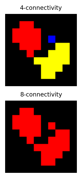
Identifying multiple objects in a binary image involves separating distinct groups of pixels that are considered ‘connected’ to one another, and then creating a ROI or label for each group. Connectivity in this sense can be defined in different ways. For example, if two pixels have the same value and are immediately beside one another (above, below, to the left or right, or diagonally adjacent) then they are said to be 8-connected, because there are 8 different neighboring locations involved. Pixels are 4-connected if they are horizontally or vertically adjacent, but not only diagonally.
The choice of connectivity can make a big difference in the number and sizes of objects found, as the example on the right shows (distinct objects are shown in different colors).
Global thresholding
The easiest way to segment an image is by applying a global threshold. This identifies pixels that are above or below a fixed threshold value, giving a binary image as the output.
For a global threshold to work, the pixels inside objects need to have higher or lower values than the other pixels. We will look at image processing tricks to overcome this limitation later, but for now we will focus on examples where we want to detect objects having values that are clearly distinct from the background – and so global thresholding could potentially work.
Thresholding using histograms
It’s possible to tell quite a lot about an image just by looking at its histogram.
Take the following example:
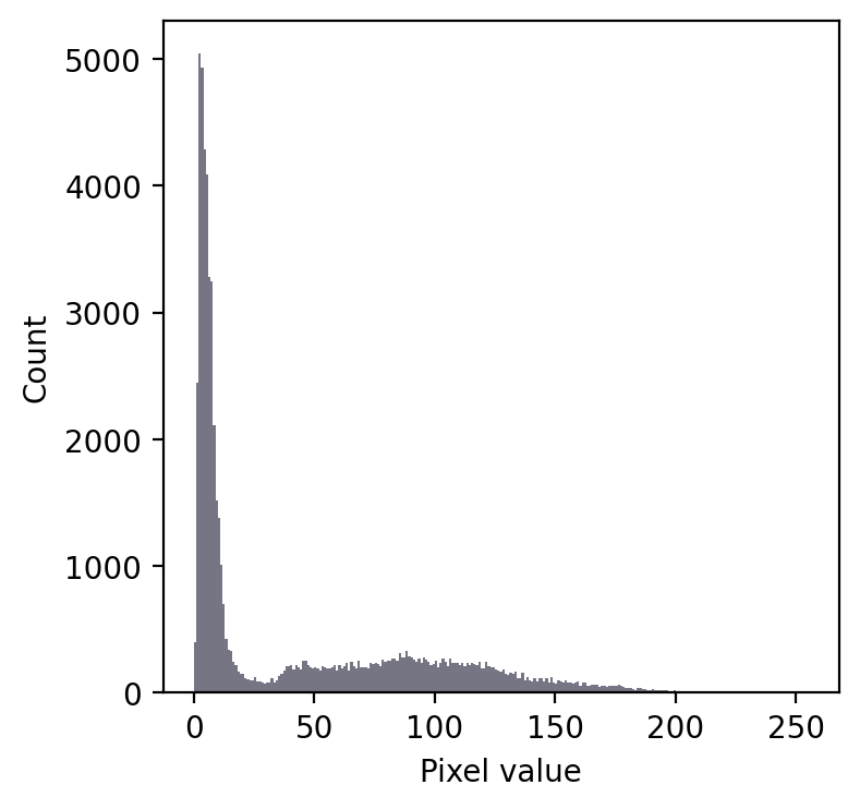
Even without seeing the image, we can make some educated guesses about its contents.
Firstly, there is a large peak to the left and a much shallower peak to the right. This suggests that there are at least two distinct regions in the image. Since the background of an image tends to contain many pixels with similar values, I would guess that we might have an image with a dark background.
In any case, a threshold around 20-25 looks like it would be a good choice to separate the regions… whatever they may be.
If we then look at the image, we can see that we have in fact got a fluorescence image depicting two nuclei. Applying a threshold of 20 does achieve a good separation of the nuclei from the background: a successful segmentation.

A simple fluorescence image containing two nuclei. We could determine a potentially useful threshold based only on looking at the histogram.
Admittedly, that was a particularly easy example. We should try a slightly harder one.
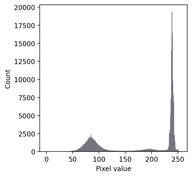
We still have a large peak, but this time it is towards the right. So I would guess a light background rather than a dark one.
But the problem is that we seem to have two shallower peaks to the left. That suggests at least three different classes of pixels in the image.
From visual inspection, we might suppose a threshold of 140 would make sense. Or perhaps around 220. It isn’t clear.
This time, we do need to look at the image to decide. Even then, there is no unambiguously ‘correct’ threshold. Rather, the one we choose depends upon whether our goal is to identify the entire leaf or rather just the darkest region.
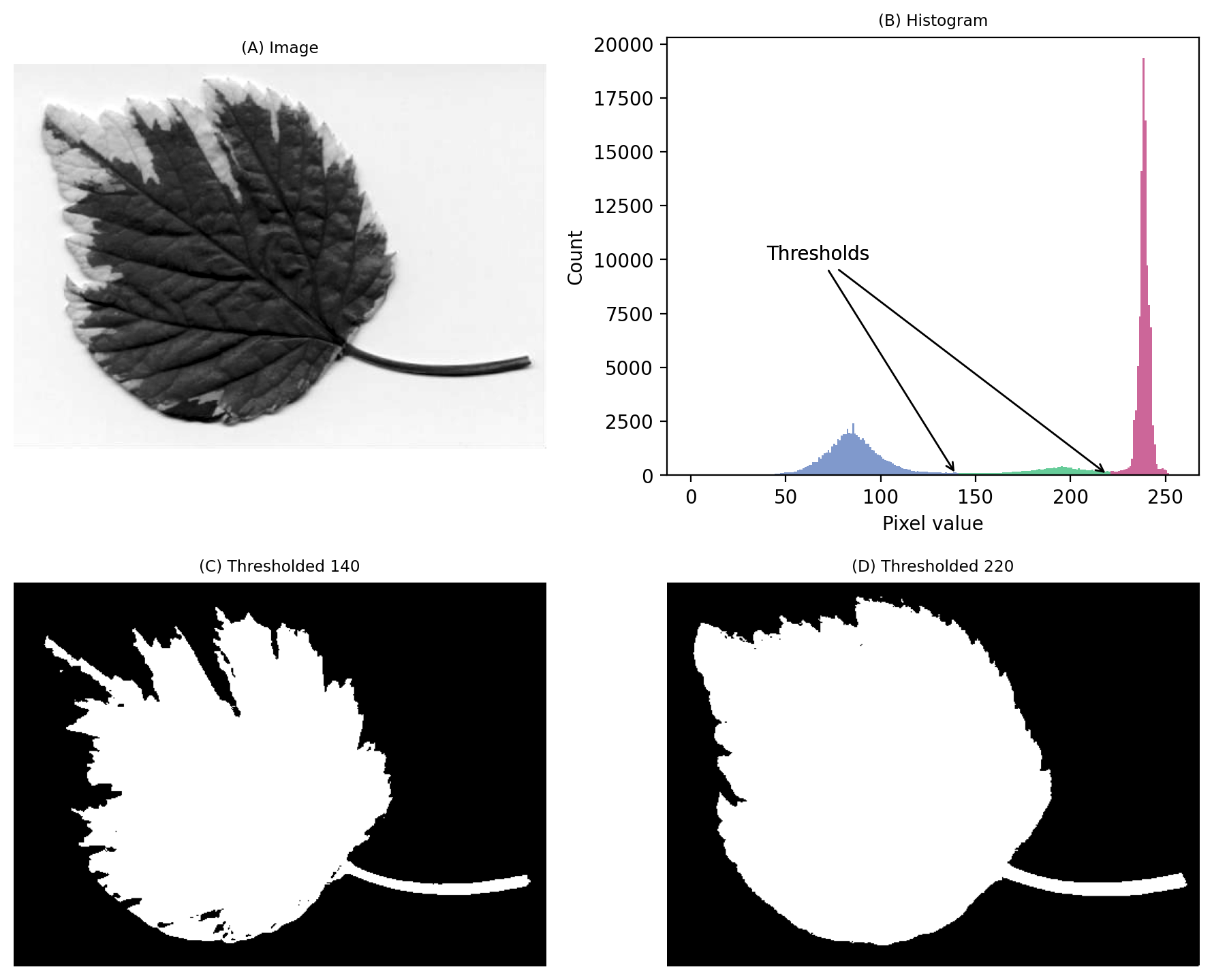
An image where evaluating the histogram suggests two candidate thresholds. The ‘correct’ threshold depends upon the desired outcome. Note that here we identify pixels below the threshold value, rather than above, because the background is lighter.
Histograms can help us choose thresholds. Histograms can be really useful when choosing threshold values – but we need to also incorporate knowledge of why we are thresholding.
In-class problems
In-class Problems Week 11
Preview of the homework image. To work on homework, please download the source of the image from Github-ScopeM-teaching Note: the image appears empty (completely white), but it is only visualisation…
For the homework, you are required to work on the image shown above (download from Github-ScopeM-teaching - do not use the image above for quantification - your results will be wrong!).
The quiz is posted on Moodle under ‘Quizzes’ and requires answers to the following questions:
Find out how many pixels are in the image blobs-homework.png?
Count the number of ‘blobs’ in blobs-homework.png, following the criteria provided below, and report the number.
Segment blobs-homework.png using thresholding (use the Intermodes algorithm to determine the threshold, then configure and run Analyze > Measure Particles).
Include partial blobs (i.e. touching the edges)
Do not perform any pre-processing on the input image before (e.g. blur) nor post-processing of outputs (e.g. separation of touching blobs)
Exclude blobs with area smaller than 100 pixels
Measure some intensity values of the image and report the numbers (in ImageJ/Fiji, use Analyze > Measure, after configuring what is measured in Analyze > Set Measurements…. Feel free to use Python or other software). We allow an error of about 5%, due to the handling of rounding by different software.
Mean intensity of image
Median intensity of image
Standard deviation of intensities of image
Measure the mean gray-scale value of all segmented blobs. We allow 10% error in case your segmentation differs from the “correct” answer in 2.
Measure the average size (number of pixels) of segmented blobs. We allow 10% error in case your segmentation differs from the “correct” answer in 2.