Linear Regression
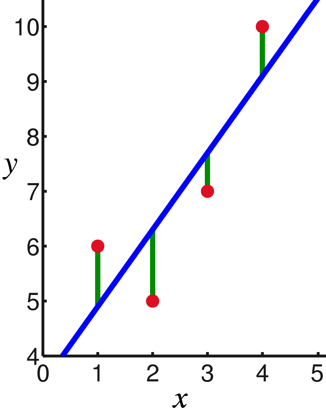
Linear regression is the modelling of the relationship between an output variable or measurement and one or more possible explanatory variables. The simplest form would be the “best-fit” line on a scatterplot, with the form:
The method for fitting the model is to minimise the total residuals in the y-axis, which can be visualised:

In R, the lm function allows you to fit this simple model.
# Linear Model
data(cars)
fit <- lm(dist ~ speed, data=cars)
summary(fit)
par(mfrow=c(2,2))
plot(fit)
The summary of the model provides a significance value based on a correlation (see below), or for a categorical variable it provides the results of a t-test for each level against the first level.
The diagnostic plots can be useful to see whether your linear model makes sense or not. You can check whether there’s a systematic error, such as your residuals scaling with your fitted values, or non-normality of the data. Points marked with values indicate outliers.
If you are working with categorial data and want to obtain a summary statistic for such variables, the anova function has a method for linear models.
# Categorical variables
data(mtcars)
fit <- lm(mpg ~ as.factor(cyl), data=mtcars)
summary(fit)
anova(fit)
Multiple Variables
The power of this method comes from the fact that it can be used for multiple explanatory variables and can therefore be used to find a model based on only the variables that matter.
We can use exactly the same functions as before by giving lm a formula including the variables we are interested in. However, when there is more than one variable there is the possibility that the two are dependent and could mislead us. To account for this we can also add an interaction term to the formula.
# Multiple variables
data(mtcars)
fit <- lm(mpg ~ as.factor(cyl) + disp, data=mtcars)
summary(fit)

# Are disp and cyl dependent?
boxplot(disp ~ cyl, data=mtcars)

# Include interaction
fit <- lm(mpg ~ as.factor(cyl) + disp + as.factor(cyl):disp, data=mtcars)
summary(fit)
Of course, we could go further and include all the variables in the data and all possible two-way, three-way, etc. interactions. How do we avoid making a model that fits perfectly but includes unnecessary variables? We can of course remove those that are shown to be insignificant, but there are sophisticated methods to better determine whether your model is the correct fit or not.
Two such methods are the Akaike Information Criteria or AIC and the Bayesian Information Criteria or BIC. In R the functions are the capitalised acronyms and they return a single value as an assessment of a model generated by lm. The smaller the value, the better the fit.
# Fitting the best model
data(mtcars)
fit_cyl <- lm(mpg ~ as.factor(cyl), data=mtcars)
fit_disp <- lm(mpg ~ disp, data=mtcars)
fit_both <- lm(mpg ~ as.factor(cyl) + disp + as.factor(cyl):disp, data=mtcars)

AIC(fit_cyl)
AIC(fit_disp)
AIC(fit_both)

# The more complex model is a better fit
Correlation
As noted above, the lm function in R determines the likelihood of a single continuous variable fit by correlation. Specifically it uses the Pearson product moment correlation coefficient. Without going into details, this is the most common parametric measure of correlation, but is not very robust. Common ways that data can mistakenly appear correlated include multimodal distributions and exponentially distributed data, and the statistic can only recognise linear relationships.
A non-parametric equivalent is the Spearman correlation, which is literally just the Pearson correlation of the ranks of the data. Another nonparametric test is the Kendall correlation, which considers whether pairs of points are concordant (i.e.: their sort order agrees) in both data sets.
In R, the cor and cor.test functions will perform these different correlation measures.
Remember though, that correlation does not mean causation.
Exercises
Load the mtcars data and build a linear model with a single variable that best explains the qsec data
Hint: to understand what each column is, use ?mtcars
Now construct the best model you can using whichever variables appear significant and applying the AIC criteria
How might you determine which factors are responsible for the variations seen between vehicles?